10.4 Square Roots in Residue Class Rings

Team-Fly

---

10.4 Square Roots in Residue Class Rings

Now that we have calculated square roots of whole numbers, or their integer parts, we turn our attention once again to residue classes, where we shall do the same thing, that is, calculate square roots. Under certain assumptions there exist square roots in residue class rings, though in general they are not uniquely determined (that is, an element may have more than one square root). Put algebraically, the question is to determine whether for an element ā Î there exist roots for which = ā. In number-theoretic notation (see Chapter 5) this would appear in congruence notation, and we would ask whether the quadratic congruence

has any solutions, and if it does, what they are.

If gcd(a, m) = 1 and there exists a solution b with b² ≡ a mod m, then a is called a quadratic residue modulo m. If there is no solution to the congruence, then a is called a quadratic nonresidue modulo m. If b is a solution to the congruence, then so is b + m, and therefore we can restrict our attention to those residues that differ modulo m.

Let us clarify the situation with the help of an example: 2 is a quadratic residue modulo 7, since 3² ≡ 9 ≡ 2 (mod 7), while 3 is a quadratic nonresidue modulo 5.

In the case that m is a prime number, then the determination of square roots modulo m is easy, and in the next chapter we shall present the functions required for this purpose. However, the calculation of square roots modulo a composite number depends on whether the prime factorization of m is known. If it is not, then the determination of square roots for large m is a mathematically difficult problem in the complexity class NP (see page 100), and it is this level of complexity that ensures the security of modern cryptographic systems.^[3] We shall return to more elucidative examples in Section 10.4.4

The determination of whether a number has the property of being a quadratic residue and the calculation of square roots are two different computational problems each with its own particular algorithm, and in the following sections we will provide explanations and implementations. We first consider procedures for determining whether a number is a quadratic residue modulo a given number. Then we shall calculate square roots modulo prime numbers, and in a later section we shall give approaches to calculating square roots of composite numbers.

10.4.1 The Jacobi Symbol

We plunge right into this section with a definition: Let p ≠ 2 be a prime number and a an integer. The Legendre symbol (say "a over p") is defined to be 1 if a is a quadratic residue modulo p and to be −1 if a is a quadratic nonresidue modulo p. If p is a divisor of a, then := 0. As a definition the Legendre then symbol does not seem to help us much, since in order to know its value we have to know whether a is a quadratic residue modulo p. However, the Legendre symbol has properties that will allow us to do calculations with it and above all to determine its value. Without going too far afield we cannot go into the theoretical background. For that the reader is referred to, for example, [Bund], Section 3.2. Nonetheless, we would like to cite some of these properties to give the reader an idea of the basis for calculation with the Legendre symbol:

1. The number of solutions of the congruence x² ≡ a (mod p) is 1 + .

2. There are as many quadratic residues as nonresidues modulo p, namely (p − 1)/2.

3. a ≡ b (mod p) ⇒ = .

4. The Legendre symbol is multiplicative: .

5. = 0

6. a^(p−1)/2 ≡ (mod p) (Euler criterion).

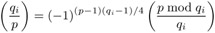
7. For an odd prime q, q ≠ p, we have = (−1)^{(p−1)(q−1)/4} (law of quadratic reciprocity of Gauss).

8. = (−1)^(p−1)/2, , = 1.

The proofs of these properties of the Legendre symbol can be found in the standard literature on number theory, for example [Bund] or [Rose].

Two ideas for calculating the Legendre symbol come at once to mind: We can use the Euler criterion (vi) and compute a^(p−1)/2 (mod p). This requires a modular exponentiation (an operation of complexity O (log³ p)). Using the reciprocity law, however, we can employ the following recursive procedure, which is based on properties (iii), (iv), (vii), and (viii).

Recursive algorithm for calculating the Legendre symbol of an integer a and an odd prime p

1. If a = 1, then = 1 (property (viii)).

2. If a is even, then (properties (iv), (viii)).

3. If a ≠ 1 and a = q₁ ... q_k is the product of odd primes q₁,..., q_k, then

   

   For each i we compute

   

   by means of steps 1 through 3 (properties (iii), (iv), and (vii)).

Before we examine the programming techniques required for computing the Legendre symbol we consider a generalization that can be carried out without the prime decomposition, such as would be required by the direct application of the reciprocity law in the version above (vii), which for large numbers takes an enormous amount of time (for the factoring problem see page 199). At that point we will be able to fall back on a nonrecursive procedure: For an integer a and an integer b = p₁ = p₂...p_k with not necessarily distinct prime factors p_i the Jacobi symbol (or Jacobi-Kronecker, Kronecker-Jacobi, or Kronecker symbol) is defined as the product of the Legendre symbols :

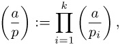
where

For the sake of completeness we set := 1 for a Î , := 1 if a = ±1, and := 0 otherwise.

If b is itself an odd prime (that is, k = 1), then the values of the Jacobi and Legendre symbols are the same. In this case the Jacobi (Legendre) symbol specifies whether a is a quadratic residue modulo b, that is, whether there is a number c with c² ≡ a mod b, in which case = 1. Otherwise, = −1 (or = 0 if a ≡ 0 mod b). If b is not a prime (that is, k > 1), then we have that a is a quadratic residue modulo b if and only if gcd(a, b) = 1 and a is a quadratic residue modulo all primes that divide b, that is, if all Legendre symbols , i = 1,..., k, have the value 1. This is clearly not equivalent to the Jacobi symbol having the value 1: Since x² ≡ 2 mod 3 has no solution, we have = −1. However, by definition, = = 1, although for x² ≡ 2 mod 9 there is likewise no solution. On the other hand, if = −1, then a is in every case a quadratic nonresidue modulo b. The relation = 0 is equivalent to gcd(a, b) ≠ 1.

From the properties of the Legendre symbol we can conclude the following about the Jacobi symbol:

1. = , and if b · c ≠ 0, then = .

2. a ≡ c mod b ⇒ = .

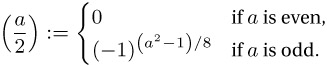
3. For odd b > 0 we have = (−1)^(b−1)/2, = (−1)^(b2−1)/8, and = 1 (see (viii) above).

4. For odd a and b with b > 0 we have the reciprocity law (see (viii) above) = (−1)^{(a−1)(b−1)/4} .

From these properties (see the above references for the proofs) of the Jacobi symbol we have the following algorithm of Kronecker, taken from [Cohe], Section 1.4, that calculates the Jacobi symbol (or, depending on the conditions, the Legendre symbol) of two integers in a nonrecursive way. The algorithm deals with a possible sign of b, and for this we set := 1 for a ≥ 0 and := −1 for a < 0.

Algorithm for calculating the Jacobi symbol of integers a and b

1. If b = 0, output 1 if the absolute value |a| of a is equal to 1; otherwise, output 0 and terminate the algorithm.

2. If a and b are both even, output 0 and terminate the algorithm. Otherwise, set v ← 0, and as long as b is even, set v ← v + 1 and b ← b/2. If now v is even, set k ← 1; otherwise, set k ← . If b < 0, then set b ← −b. If a < 0, set k ← −k (cf. (iii)).

3. If a = 0, output 0 if b > 1, otherwise k, and terminate the algorithm. Otherwise, set v ← 0, and as long as a is even, set v ← v + 1 and a ← a/2. If now v is odd, set k ← · k (cf. (iii)).

4. Set k ← (−1)^{(a−1)(b−1)/4} · k, r ← |a|, a ← b mod r, b ← r, and go to step 3 (cf. (ii) and (iv)).

The run time of this procedure is O (log² N), where N ≥ a, b represents an upper bound for a and b. This is a significant improvement over what we achieved with the Euler criterion. The following tips for the implementation of the algorithm are given in Section 1.4 of [Cohe].

• The values and in steps 2 and 3 are best computed with the aid of a prepared table.

• The value (−1)^{(a−1)(b−1)/4} · k in step 4 can be efficiently determined with the C expression if(a&b&2) k = −k, where & is bitwise AND.

In both cases the explicit computation of a power can be avoided, which of course has a positive effect on the total run time.

We would like to clarify the first tip with the help of the following considerations: If k in step 2 is set to the value , then a is odd. The same holds for b in step 3. For odd a we have

or

so that 8 is a divisor of (a − 1)(a + 1) = a² − 1. Thus is an integer. Furthermore, we have (this can be seen by placing the representation a = k · 8 + r in the exponent). The exponent must therefore be determined only for the four values a mod 8 = ±1 and ±3, for which the results are 1, −1, −1, and 1. These are placed in a vector {0, 1, 0, −1, 0, −1, 0, 1}, so that by knowing a mod 8 one can access the value of . Observing that a mod 8 can be represented by the expression a & 7, where again & is binary AND, then the calculation of the power is reduced to a few fast CPU operations. For an understanding of the second tip we note that (a & b & 2) ≠ 0 if and only if (a − 1)/2 and (b − 1)/2, and hence (a − 1)(b − 1)/4 , are odd.

Finally, we use the auxiliary function twofact_l(), which we briefly introduce here, for determining v and b in step 2, for the case that b is even, as well as in the analogous case for the values v and a in step 3. The function twofact_l() decomposes a CLINT value into a product consisting of a power of two and an odd factor.

Function:	decompose a CLINT object a = 2ku with odd u
Syntax:	int twofact_l (CLINT a_l, CLINT b_l);
Input:	a_l (operand)
Output:	b_l (odd part of a_l)
Return:	k (logarithm to base 2 of the two-part of a_l)

 int twofact_l (CLINT a_l, CLINT b_l) {   int k = 0;   if (EQZ_L (a_l))     {       SETZERO_L (b_l);       return 0;     }   cpy_l (b_l, a_l);   while (ISEVEN_L (b_l))     {       shr_l (b_l);       ++k;     }   return k; } 

Thus equipped we can now create an efficient function jacobi_l() for calculating the Jacobi symbol.

Function:	calculate the Jacobi symbol of two CLINT objects
Syntax:	int jacobi_l (CLINT aa_l, CLINT bb_l);
Input:	aa_l, bb_l (operands)
Return:	±1 (value of the Jacobi symbol of aa_l over bb_l)

 static int tab2[] = 0, 1, 0, −1, 0, −1, 0, 1; int jacobi_l (CLINT aa_l, CLINT bb_l) {   CLINT a_l, b_l, tmp_l;   long int k, v; 

Step 1: The case bb_l = 0.

   if (EQZ_L (bb_l))     {       if (equ_l (aa_l, one_l))          {            return 1;          }       else          {            return 0;          }     } 

Step 2: Remove the even part of bb_l.

   if (ISEVEN_L (aa_l) && ISEVEN_L (bb_l))     {       return 0;     }   cpy_l (a_l, aa_l);   cpy_l (b_l, bb_l);   v = twofact_l (b_l, b_l);   if ((v & 1) == 0)    /* v even? */     {       k = 1;     }   else     {       k = tab2[*LSDPTR_L (a_l) & 7];  /* *LSDPTR_L (a_l) & 7 == a_l % 8 */     } 

Step 3: If a_l = 0, then we are done. Otherwise, the even part of a_l is removed.

   while (GTZ_L (a_l))     {       v = twofact_l (a_l, a_l);       if ((v & 1) != 0)          {            k = tab2[*LSDPTR_L (b_l) & 7];          } 

Step 4: Application of the quadratic reciprocity law.

       if (*LSDPTR_L (a_l) & *LSDPTR_L (b_l) & 2)          {            k = -k;          }       cpy_l (tmp_l, a_l);       mod_l (b_l, tmp_l, a_l);       cpy_l (b_l, tmp_l);     }   if (GT_L (b_l, one_l))     {       k = 0;     }   return (int) k; } 

10.4.2 Square Roots Modulo p^k

We now have an idea of the property possessed by an integer of being or not being a quadratic residue modulo another integer, and we also have at our disposal an efficient program to determine which case holds. But even if we know whether an integer a is a quadratic residue modulo an integer n, we still cannot compute the square root of a, especially not in the case where n is large. Since we are modest, we will first attempt this feat for those n that are prime. Our task, then, is to solve the quadratic congruence

(10.11) 

where we assume that p is an odd prime and a is a quadratic residue modulo p, which guarantees that the congruence has a solution. We shall distinguish the two cases p ≡ 3 mod 4 and p ≡ 1 mod 4. In the former, simpler, case, x := a^(p+1)/4 mod p solves the congruence, since

(10.12) 

where for a^(p−1)/2 ≡ ≡ 1 mod p we have used property (vi) of the Legendre symbol, the Euler criterion, cited above.

The following considerations, taken from [Heid], lead to a general procedure for solving quadratic congruences, and in particular for solving congruences of the second case, p ≡ 1 mod 4: We write p − 1 = 2^kq, with k ≥ 1 and q odd, and we look for an arbitrary quadratic nonresidue n mod p by choosing a random number n with 1 ≤ n < p and calculating the Legendre symbol . This has value −1 with probability , so that we should find such an n relatively quickly. We set

(10.13)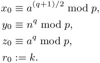 

Since by Fermat's little theorem we have a^(p−1)/2 ≡ x^2(p−1)/2 ≡ x^p−1 ≡ 1 mod p for a and for a solution x of (10.11), and since additionally, for quadratic nonresidues n we have n^(p−1)/2 ≡ −1 mod p (cf. (vi), page 218), we have

(10.14)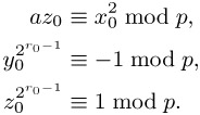 

If z₀ ≡ 1 mod p, then x₀ is already a solution of the congruence (10.11). Otherwise, we recursively define numbers x_i, y_i, z_i, r_i such that

(10.15)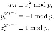 

and r_i > r_i−1. After at most k steps we must have z_i ≡ 1 mod p and that x_i is a solution to (10.11). To this end we choose m₀ as the smallest natural number such that ≡ 1 mod p, whereby m₀ ≤ r₀ − 1. We set

(10.16)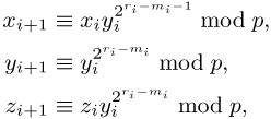 

with r_i+1 := m_i := min { m ≥ 1 | ≡ 1 mod p }. Then

(10.17)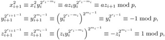 

since ≡ ≡ 1 mod p, and therefore by the minimality of m_i only ≡ −1 mod p is possible.

We have thus proved a solution procedure for quadratic congruence, on which the following algorithm of D. Shanks is based (presented here as in [Cohe], Algorithm 1.5.1).

Algorithm for calculating square roots of an integer a modulo an odd prime p

1. Write p − 1 = 2^kq, q odd. Choose random numbers n until = −1.

2. Set x ← a^(q−1)/2 mod p, y ← n^q mod p, z ← a · x² mod p, x ← a · x mod p, and r ← k.

3. If z ≡ 1 mod p, output x and terminate the algorithm. Otherwise, find the smallest m for which ≡ 1 mod p. If m = r, then output the information that a is not a quadratic residue p and terminate the algorithm.

4. Set t ← mod p, y ← t² mod p, r ← m mod p, x ← x · t mod p, z ← z · y mod p, and go to step 3.

It is clear that if x is a solution of the quadratic congruence, then so is −x mod p, since (−x)² ≡ x² mod p.

Out of practical considerations in the following implementation of the search for a quadratic nonresidue modulo p we shall begin with 2 and run through all the natural numbers testing the Legendre symbol in the hope of finding a nonresidue in polynomial time. In fact, this hope would be a certainty if we knew that the still unproved extended Riemann hypothesis were true (see, for example, [Bund], Section 7.3, Theorem 12, or [Kobl], Section 5.1, or [Kran], Section 2.10). To the extent that we doubt the truth of the extended Riemann hypothesis the algorithm of Shanks is probabilistic.

For the practical application in constructing the following function proot_l() we ignore these considerations and simply expect that the calculational time is polynomial. For further details see [Cohe], pages 33 f.

Function:	compute the square root of a modulo p
Syntax:	int proot_l (CLINT a_l, CLINT p_l, CLINT x_l);
Input:	a_l, p_l (operands, p_l > 2 a prime)
Output:	x_l (square root of a_l modulo p_l)
Return:	0 if a_l is a quadratic residue modulo p_l −1 otherwise

 int proot_l (CLINT a_l, CLINT p_l, CLINT x_l) {   CLINT b_l, q_l, t_l, y_l, z_l;   int r, m;   if (EQZ_L (p_l) || ISEVEN_L (p_l))     {       return −1;     } 

If a_l == 0, the result is 0.

   if (EQZ_L (a_l))     {       SETZERO_L (x_l);       return 0;     } 

Step 1: Find a quadratic nonresidue.

   cpy_l (q_l, p_l);   dec_l (q_l);   r = twofact_l (q_l, q_l);   cpy_l (z_l, two_l);   while (jacobi_l (z_l, p_l) == 1)     {       inc_l (z_l);     }   mexp_l (z_l, q_l, z_l, p_l); 

Step 2: Initialization of the recursion.

   cpy_l (y_l, z_l);   dec_l (q_l);   shr_l (q_l);   mexp_l (a_l, q_l, x_l, p_l);   msqr_l (x_l, b_l, p_l);   mmul_l (b_l, a_l, b_l, p_l);   mmul_l (x_l, a_l, x_l, p_l); 

Step 3: End of the procedure; otherwise, find the smallest m such that ≡ 1 mod p.

   mod _l (b_l, p_l, q_l);   while (!equ_l (q_l, one_l))     {       m = 0;       do          {            ++m;            msqr_l (q_l, q_l, p_l);          }       while (!equ_l (q_l, one_l));       if (m == r)          {            return −1;          } 

Step 4: Recursion step for x, y, z, and r.

       mexp2_l (y_l, (ULONG)(r − m − 1), t_l, p_l);       msqr_l (t_l, y_l, p_l);       mmul_l (x_l, t_l, x_l, p_l);       mmul_l (b_l, y_l, b_l, p_l);       cpy_l (q_l, b_l);       r = m;       }     return 0;   } 

The calculation of roots modulo prime powers p^k can now be accomplished on the basis of our results modulo p. To this end we first consider the congruence

(10.18) 

based on the following approach: Given a solution x₁ of the above congruence x² ≡ a mod p we set x := x₁ + p · x², from which follows

From this we deduce that for solving (10.18) we will be helped by a solution x₂ of the linear congruence

Proceeding recursively one obtains in a number of steps a solution of the congruence x² ≡ a mod p^k for any k Î .

10.4.3 Square Roots Modulo n

The ability to calculate square roots modulo a prime power is a step in the right direction for what we really want, namely, the solution of the more general problem x² ≡ a mod n for a composite number n. However, we should say at once that the solution of such a quadratic congruence is in general a difficult problem. In principle, it is solvable, but it requires a great deal of computation, which grows exponentially with the size of n: The solution of the congruence is as difficult (in the sense of complexity theory) as factorization of the number n. Both problems lie in the complexity class NP (cf. page 100). The calculation of square roots modulo composite numbers is therefore related to a problem for whose solution there has still not been discovered a polynomial-time algorithm. Therefore, for large n we cannot expect to find a fast solution to this general case.

Nonetheless, it is possible to piece together solutions of quadratic congruences y² ≡ a mod r and z² ≡ a mod s with relatively prime numbers r and s to obtain a solution of the congruence x² ≡ a mod rs. Here we will be assisted by the Chinese remainder theorem:

• Given congruences x ≡ a_i mod m_i with natural numbers m₁,..., m_r that are pairwise relatively prime (that is, gcd (m_i, m_j) = 1 for i ≠ j)and integers a₁,..., a_r, there exists a common solution to the set of congruences, and furthermore, such a solution is unique modulo the product m₁ · m₂ ··· m_r.

We would like to spend a bit of time in consideration of the proof of this theorem, for it contains hidden within itself in a remarkable way the promised solution: We set m := m₁ · m₂ ··· m_r and := m/m_j. Then is an integer and gcd (,m^j) = 1. From Section 10.2 we know that that there exist integers u_j and v_j with 1 = u_j + m_jv_j, that is, u_j ≡ 1 mod m_j, for j = 1,...,r and how to calculate them.

We then form the sum

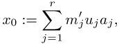
and since u_j ≡ 0 mod m_i for i ≠ j, we obtain

(10.19) 

and in this way have constructed a solution to the problem. For two solutions x₀ ≡ a_i mod m_i and x₁ ≡ a_i mod m_i we have x₀ ≡ x₁ mod m_i. This is equivalent to the difference x₀ − x₁ being simultaneously divisible by all m_i, that is, by the least common multiple of the m_i. Due to the pairwise relative primality of the m_i, we have that the least common multiple is, in fact, the product of the m_i, so that finally, we have that x₀ ≡ x₁ mod m holds.

We now apply the Chinese remainder theorem to obtain a solution of x² ≡ a mod rs with gcd(r, s) = 1, where r and s are distinct odd primes and neither r nor s is a divisor of a, on the assumption that we have already obtained roots of y² ≡ a mod r and z² ≡ a mod s. We now construct as above a common solution to the congruences

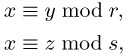
by

where 1 = ur + vs is the representation of the greatest common divisor of r and s. We thus have ≡ a mod r and ≡ a mod s, and since gcd(r, s) = 1, we also have ≡ a mod rs, and so we have found a solution of the above quadratic congruence. Since as shown above every quadratic congruence modulo r and modulo s possesses two solutions, namely ±y and ±z, the congruence modulo rs has four solutions, obtained by substituting in ±y and ±z above:

(10.20) 

(10.21) 

(10.22) 

(10.23) 

We have thus found in principle a way to reduce the solution of quadratic congruences

with n odd to the case x² ≡ a mod p for primes p. For this we determine the prime factorization n = and then calculate the roots modulo the p_i, which by the recursion in Section 10.4.2 can be used to obtain solutions of the congruences x₂ ≡ a mod . As the crowning glory of all this we then assemble these solutions with the help of the Chinese remainder theorem into a solution of x² ≡ a mod n. The function that we give takes this path to solving a congruence x² ≡ a mod n. However, it assumes the restricted hypothesis that n = p · q is the product of two odd primes p and q, and first calculates solutions x₁ and x₂ of the congruences

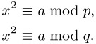
From x₁ and x₂ we assemble according to the method just discussed the solutions to the congruence

and the output is the smallest square root of a modulo pq.

Function:	calculate the square root of a modulo p · q for odd primes p, q
Syntax:	int root_l (CLINT a_l, CLINT p_l, CLINT q_l, CLINT x_l);
Input:	a_l, p_l, q_l (operands, primes p_l, q_l > 2)
Output:	x_l (square root of a_l modulo p_l)
Return:	0 if a_l is a quadratic residue modulo p_l * q_l −1 otherwise

 int root_l (CLINT a_l, CLINT p_l, CLINT q_l, CLINT x_l)  {   CLINT x0_l, x1_l, x2_l, x3_l, xp_l, xq_l, n_l;   CLINTD u_l, v_l;   clint *xptr_l;   int sign_u, sign_v; 

Calculate the roots modulo p_l and q_l with the function proot_l(). If a_l == 0, the result is 0.

 if (0 != proot_l (a_l, p_l, xp_l) || 0 != proot_l (a_l, q_l, xq_l))   {     return −1;   } if (EQZ_L (a_l))   {     SETZERO_L (x_l);     return 0;   } 

For the application of the Chinese remainder theorem we must take into account the signs of the factors u_l and v_l, represented by the auxiliary variables sign_u and sign_v, which assume the values calculated by the function xgcd_l(). The result of this step is the root x₀.

 mul_l (p_l, q_l, n_l); xgcd_l (p_l, q_l, x0_l, u_l, &sign_u, v_l, &sign_v); mul_l (u_l, p_l, u_l); mul_l (u_l, xq_l, u_l); mul_l (v_l, q_l, v_l); mul_l (v_l, xp_l, v_l); sign_u = sadd (u_l, sign_u, v_l, sign_v, x0_l); smod (x0_l, sign_u, n_l, x0_l); 

Now we calculate the roots x₁, x₂, and x₃.

 sub_l (n_l, x0_l, x1_l); msub_l (u_l, v_l, x2_l, n_l); sub_l (n_l, x2_l, x3_l); 

The smallest root is returned as result.

 xptr_l = MIN_L (x0_l, x1_l); xptr_l = MIN_L (xptr_l, x2_l); xptr_l = MIN_L (xptr_l, x3_l);   cpy_l (x_l, xptr_l);   return 0; } 

From this we can now easily deduce an implementation of the Chinese remainder theorem by taking the code sequence from the above function and extending it by the number of congruences that are to be simultaneously solved. Such a procedure is described in the following algorithm, due to Garner (see [MOV], page 612), which has an advantage with respect to the application of the Chinese remainder theorem in the above form in that reduction must take place only modulo the m_i, and not modulo m = m₁m₂ ··· m_r. This results in a significant savings in computing time.

Algorithm 1 for a simultaneous solution of a system of linear congruences

x ≡ a_i mod m_i, 1 ≤ i ≤ r, with gcd (m_i, m_j) = 1 for i ≠ j

1. Set u ← a₁, x ← u, and i ← 2.

2. Set C_i ← 1, j ← 1.

3. Set u ← mod m_i (computed by means of the extended Euclidean algorithm; see page 179) and C_i ← uC_i mod m_i.

4. Set j ← j + 1; if j ≤ i − 1, go to step 3.

5. Set u ← (a_i − x)C_i mod m_i, and x ← x + u m_j.

6. Set i ← i + 1; if i ≤ r, go to step 2. Otherwise, output x.

It is not obvious that the algorithm does what it is supposed to, but this can be shown by an inductive argument. To this end let r = 2. In step 5 we then have

It is seen at once that x ≡ a₁ mod m₁. However, we also have

To finish the induction by passing from r to r + 1 we assume that the algorithm returns the desired result x_r for some r ≥ 2, and we append a further congruence x ≡ a_r+1 mod m_r+1. Then by step 5 we have

Here we have x ≡ x_r ≡ a_i mod m_i for i = 1,...,r according to our assumption. But we also have

which completes the proof.

For the application of the Chinese remainder theorem in programs one function would be particularly useful, one that is not dependent on a predetermined number of congruences, but rather allows the number of congruences to be specified at run time. This method is supported by an adaptation of the above construction procedure, which does not, alas, have the advantage that reduction need take place only modulo m_i, but it does make it possible to process the parameters a_i and m_i of a system of congruences with i = 1, ..., r with variable r with a constant memory expenditure. Such a solution is contained in the following algorithm from [Cohe], Section 1.3.3.

Algorithm 2 for calculating a simultaneous solution of a system of linear congruences x ≡ a_i mod m_i, 1 ≤ i ≤ r, with gcd (m_i, m_j) = 1 for i ≠ j

1. Set i ← 1, m ← m₁, and x ← a₁.

2. If i = r, output x and terminate the algorithm. Otherwise, increase i ← i + 1 and calculate u and v with 1 = um + vm_i using the extended Euclidean algorithm (cf. page 177).

3. Set x ← uma_i + vm_ix, m ← mm_i, x ← x mod m and go to step 2.

The algorithm immediately becomes understandable if we carry out the computational steps for three equations x = a_i mod m_i, i = 1, 2, 3: For i = 2 we have in step 2

and in step 3

In the next pass through the loop with i = 3 the parameters a₃ and m₃ are processed. In step 2 we then have

and in step 3

The summands u₂m₁m₂a₃and v₂m₃u₁m₁a₂ disappear in forming the residue x₂ modulo m₁; furthermore, v₂m₃ ≡ v₁m₂ ≡ 1 mod m₁ by construction, and thus x₂ ≡ a₁ mod m₁ solves the first congruence. Analogous considerations lead us to see that x₂ also solves the remaining congruences.

We shall implement this inductive variant of the construction principle according to the Chinese remainder theorem in the following function chinrem_l(), whose interface enables the passing of coefficients of a variable number of congruences. For this a vector with an even number of pointers to CLINT objects is passed, which in the order a₁, m₁, a₂, m₂, a₃, m₃,... are processed as coefficients of congruences x ≡ a_i mod m_i. Since the number of digits of the solution of a congruence system x ≡ a_i mod m_i is of order Σ_i log (m_i), the procedure is subject to overflow in its dependence on the number of congruences and the size of the parameters. Therefore, such errors will be noted and indicated in the return value of the function.

Function:	solution of linear congruences with the Chinese remainder theorem
Syntax:	int chinrem_l (int noofeq, clint **coeff_l, CLINT x_l);
Input:	noofeq (number of congruences) coeff_l (vector of pointers to CLINT coefficients ai, mi of congruences x ≡ ai mod mi, i = 1,...,noofeq)
Output:	x_l (solution of the system of congruences)
Return:	E_CLINT_OK if all is ok E_CLINT_OFL if overflow 1 if noofeq is 0 2 if mi are not pairwise relatively prime

 int chinrem_l (unsigned int noofeq, clint** coeff_l, CLINT x_l) {   clint *ai_l, *mi_l;   CLINT g_l, u_l, v_l, m_l;   unsigned int i;   int sign_u, sign_v, sign_x, err, error = E_CLINT_OK;   if (0 == noofeq)     {       return 1;     } 

Initialization: The coefficients of the first congruence are taken up.

 cpy_l (x_l, *(coeff_l++)); cpy_l (m_l, *(coeff_l++)); 

If there are additional congruences, that is, if no_of_eq > 1, the parameters of the remaining congruences are processed. If one of the mi_l is not relatively prime to the previous moduli occurring in the product m_l, then the function is terminated and 2 is returned as error code.

   for (i = 1; i < noofeq; i++)     {       ai_l = *(coeff_l++);       mi_l = *(coeff_l++);       xgcd_l (m_l, mi_l, g_l, u_l, &sign_u, v_l, &sign_v);       if (!EQONE_L (g_l))          {            return 2;          } 

In the following an overflow error is recorded. At the end of the function the status is indicated in the return of the error code stored in error.

       err = mul_l (u_l, m_l, u_l);       if (E_CLINT_OK == error)          {            error = err;          }       err = mul_l (u_l, ai_l, u_l);       if (E_CLINT_OK == error)          {            error = err;          }       err = mul_l (v_l, mi_l, v_l);       if (E_CLINT_OK == error)          {            error = err;          }       err = mul_l (v_l, x_l, v_l);       if (E_CLINT_OK == error)          {            error = err;          } 

We again use our auxiliary functions sadd() and smod(), which take care of the signs sign_u and sign_v (or sign_x) of the variables u_l and v_l (or x_l).

       sign_x = sadd (u_l, sign_u, v_l, sign_v, x_l);       err = mul_l (m_l, mi_l, m_l);       if (E_CLINT_OK == error)          {            error = err;          }       smod (x_l, sign_x, m_l, x_l);     }   return error; } 

10.4.4 Cryptography with Quadratic Residues

We come now to the promised (on page 188) examples for the cryptographic application of quadratic residues and their roots. To this end we consider first the encryption procedure of Rabin and then the identification schema of Fiat and Shamir.^[4]

The encryption procedure published in 1979 by Michael Rabin (see [Rabi]) depends on the difficulty of calculating square roots in . Its most important property is the provable equivalence of this calculation to the factorization problem (see also [Kran], Section 5.6). Since for encryption the procedure requires only a squaring modulo n, it is simple to implement, as the following demonstrates.

Rabin key generation

1. Ms. A generates two large primes p ≈ q and computes n = p · q.

2. Ms. A publishes n as a public key and uses the pair <p, q> as private key.

With the public key n_A a correspondent Mr. B can encode a message M Î in the following way and send it to Ms. A.

Rabin encryption

1. Mr. B computes C := M² mod n_A with the function msqr_l() on page 75 and sends the encrypted text C to A.

2. To decode the message, A computes from C the four square roots M_i modulo n_A, i = 1,...,4, with the aid of the function root_l() (cf. page 201), which here is modified so that not only the smallest but all four square roots are output.^[5] One of these roots is the plain text M.

Ms. A now has the problem of deciding which of the four roots M_i, represents the original plain text M. If prior to encoding the message B adds some redundant material, say a repetition of the last r bits, and informs A of this, then A will have no trouble in choosing the right text, since the probability that one of the other texts will have the same identifier is very slight.

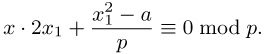
Furthermore, redundancy prevents the following attack strategy against the Rabin procedure: If an attacker X chooses at random a number R Î and is able to obtain from A one of the roots R_i of X := R² mod n_A (no matter how he or she may motivate A to cooperate), then R_i ≢ ±R mod n_A will hold with probability .

From n_A = p · q | ( − R²) = (R_i − R) (R_i + R) ≠ 0, however, one would have 1 ≠ gcd (R − R_i, n_A) Î { p, q }, and X would have broken the code with the factorization of n_A (cf. [Bres], Section 5.2). On the other hand, if the plain text is provided with redundancy, then A can always recognize which root represents a valid plain text. Then A would at most reveal R (on the assumption that R had the right format), which for Mr. or Ms. X, however, would be useless.

The avoidance of deliberate or accidental access to the roots of a pretended cipher text is a necessary condition for the use of the procedure in the real world.

The following example of the cryptographic application of quadratic residues deals with an identification schema published in 1986 by Amos Fiat and Adi Shamir. The procedure, conceived especially for use in connection with smart cards, uses the following aid: Let I be a sequence of characters with information for identifying an individual A, let m be the product of two large primes p and q, and let f (Z, n) → be a random function that maps arbitrary finite sequences of characters Z and natural numbers n in some unpredictable fashion to elements of the residue class ring . The prime factors p and q of the modulus m are known to a central authority, but are otherwise kept secret. For the identity represented by I and a yet to be determined k Î the central authority has now the task of producing key components as follows.

Algorithm for key generation in the Fiat-Shamir procedure

1. Compute numbers v_i = f(I, i) Î for some i ≥ k Î .

2. Choose k different quadratic residues from among the v_i and compute the smallest square roots of in .

3. Store the values I and securely against unauthorized access (such as in a smart card).

For generating keys we can use our functions jacobi_l() and root_l(); the function f can be constructed from one of the hash functions from Chapter 16, such as RIPEMD-160. As Adi Shamir once said at a conference, "Any crazy function will do."

With the help of the information stored by the central authority on the smart card Ms. A can now authenticate herself to a communication partner Mr. B.

Protocol for authentication à la Fiat-Shamir

1. A sends I and the numbers i_j, j = 1,..., k, to B.

2. B generates = f (I, i_j) Î for j = 1,..., k. The following steps 3–6 are repeated for τ = 1,...,t (for a value t Î yet to be determined):

3. A chooses a random number r_τ Î and sends x_τ = to B.

4. B sends a binary vector to A.

5. A sends numbers y_τ := r_τ s_i Î to B.

6. B verifies that x_τ = v_i.

If A truly possesses the values , then in step 6

holds (all calculations are in ), and A thereby has proved her identity to B. An attacker who wishes to assume the identity of A can with probability 2^−kt guess the vectors that B will send in step 4, and as a precaution in step 3 send the values x_τ = v_i to B; for k = t = 1, for example, this would give the attacker an average hit number of . Thus the values of k and t should be chosen such that an attacker has no realistic probability of success and such that furthermore—depending on the application—suitable values result for

• the size of the secret key;

• the set of data to be exchanged between A and B;

• the required computer time, measured as the number of multiplications.

Such parameters are given in [Fiat] for various values of k and t with kt = 72.

All in all, the security of the procedure depends on the secure storage of the values , on the choice of k and t, and on the factorization problem: Anyone who can factor the modulus m into the factors p and q can compute the secret key components , and the procedure has been broken. It is a matter, then, of choosing the modulus in such a way that it is not easily factorable. In this regard the reader is again referred to Chapter 16, where we discuss the generation of RSA moduli, subject to the same requirements.

A further security property of the procedure of Fiat and Shamir is that A can repeat the process of authentication as often as she wishes without thereby giving away any information about the secret key values. Algorithms with such properties are called zero knowledge processes (see, for example, [Schn], Section 32.11).

^[3]The analogy between mathematical and cryptographic complexity should be approached with caution: In [Rein] we are informed that the question of whether P ≠ NP has little relevance in cryptographic practice. A polynomial algorithm for factorization with running time O (n²⁰) would still be insuperable for even relatively small values of n, while an exponential algorithm with running time would conquer even relatively large moduli. The security of cryptographic procedures in practice is really not dependent on whether P and NP are the same, despite the fact that one often sees precisely this formulation.

^[4]For the fundamental concepts necessary for an understanding of asymmetric cryptography the reader is again referred to Chapter 16.

^[5]We may assume that gcd (M, n_A) = 1 and that therefore there really exist four distinct roots of C. Otherwise, the sender B could factor the modulus n_A of the receiver A by calculating gcd (M, n_A). This, of course, is not the way a public key system should operate.

---

Team-Fly