Section 26. MSAAttribute

26. MSAAttribute

Overview

Process variation affects how resulting products and services appear to Customers. However, what you (and ultimately the Customer) see as the appearance usually does not include only the variability in the entity itself, but also some variation from the way the entity is measured. A simple example of this is to pick up a familiar object, such as this book. If you were to judge if the lettering on this page was "crisp" enough and then you handed the same page to three other people, it is highly likely that there would be a difference in answers amongst everyone. It is also likely that if someone handed you the same page later (without you knowing it was the same page) and asked you to measure it again, you would come to a different answer or conclusion. The page itself has not changed; the difference in answers is purely due to the Measurement System and specifically errors within it. The higher the Measurement Error, the harder it is to understand the true process capability and behavior.

Thus, it is crucial to analyze Measurement Systems before embarking on any Process Improvement activities.

The sole purpose of a Measurement System in Lean Sigma is to collect the right data to answer the questions being asked. To do this, the Team must be confident in the integrity of the data being collected. To confirm Data Integrity the Team must know

• The type of data

• If the available data is usable

• If the data is suitable for the project

• If it is not suitable, whether it can be made usable

• How the data can be audited

• If the data is trustworthy

To answer these questions, Data Integrity is broken down into two elements:

• Validity. Is the "right" aspect of the process being measured? The data might be from a reliable method or source, but still not match the operational definitions established for the project.

And after Validity is confirmed (some mending of the Measurement System might be required first):

• Reliability. Is the valid measurement system producing good data? This considers the accuracy and consistency of the data.

Validity is covered in the section "MSAValidity" in this chapter. Reliability is dependent on the data type. Attribute Measurement Systems are covered in this section; Continuous Measurement Systems are covered in "MSAContinuous" in this chapter.

An Attribute MSA study is the primary tool for assessing the reliability of a qualitative measurement system. Attribute data has less information content than variables data, but often it is all that's available and it is still important to be diligent about the integrity of the measurement system.

As with any MSA, the concern is whether the Team can rely on the data coming from the measurement system. To understand this better it is necessary to understand the purpose of such a system. Attribute inspection generally does one of three things:

• Classifies an entity as either Conforming or Nonconforming

• Classifies an entity into one of multiple categories

• Counts the number of "non-conformities" per entity inspected

Thus, a "perfect" Attribute Measurement System would

• Correctly classify every entity

• Always produce a correct count of an entity's non-conformities

Some attribute inspections require little judgment because the correct answer is obvious; for example, in destructive test results, the entity either broke or remained intact. In the majority of cases (typically where no destruction occurs), however, it is extremely subjective. For such a system, if many appraisers (the generic MSA terminology for those doing the measurement) are evaluating the same thing they need to agree

• With each other

• With themselves

• With an expert opinion

In an Attribute MSA, an audit of the Measurement System is done using 23 appraisers and multiple entities to appraise. Each appraiser and an "expert" evaluate every entity at least twice and from the ensuing data the tool determines

• Percentage overall agreement

• Percentage agreement within appraisers (Repeatability)

• Percentage agreement between appraisers (Reproducibility)

• Percentage agreement with known standard (Accuracy)

• Kappa (how much better the measurement system is than random chance)

Logistics

Conducting an Attribute MSA is all about careful planning and data collection. This is certainly a Team sport because at least two appraisers are required, along with an expert (if one exists), and it is unlikely that Belts apply the Measurement System in their regular job (i.e., the Belt almost certainly won't be one of the appraisers used in the MSA).

Planning the MSA takes about two hours, which usually includes a brief introduction to the tool made by the Belt to the rest of the Team and sometimes to the appraisers. Data collection (conducting the appraisals themselves) can take anywhere between an hour and a week, depending on the complexity of the measurement.

Roadmap

The roadmap to planning, data collection, and analysis is as follows:

Step 1.	Identify the metric and agree within the Team on its Operational Definition (see "KPOVs and Data" in this chapter). Often the exact Measurement System in question isn't immediately obvious. For example, in many transactional service processes, it could be the initial writing of the line items to an order, the charging of the order to a specific account, or the translation of the charges into a bill. Each of these might involve a separate classification step.
Step 2.	Identify the defects and classifications for what makes an entity defective. These should be mutually exclusive (a defect cannot fall into two categories) and exhaustive (an entity must fall into at least one category, which typically means use of a category "Defect Free"). If done correctly every entity must fall into one and only one category and all defect categories should be treated equally (there should be no appraiser bias for one defect type over another).
Step 3.	Select samples to be used in the MSA. From 30 to 50 samples are necessary, and they should span the normal extremes of the process with regards to the attribute being measured. Entities to be measured should be independent from one another. The majority of the samples should be from the "gray" areas, whereas some are clearly good and clearly bad. For example, for a sample of 30 units, five units might be clearly defective (a single, large defect or enough smaller ones to be an obvious reject), five units might be clearly acceptable (everything correct), and the remaining samples would vary in quantity and type of defects.
Step 4.	Select 23 appraisers to conduct the MSA. These should be people who normally conduct the assessment.
Step 5.	Perform the appraisal. Randomly provide the samples to one appraiser (without him knowing which sample it is or the other appraisers witnessing the appraisal) and have him rate the item. After the first appraiser has reviewed all items, repeat with the remaining appraisers. Appraisers must inspect and classify independently. After all appraisers have rated each item, repeat the whole process for one additional trial.
Step 6.	Conduct an expert appraisal or complete a comparison to a Standard. In Step 5 the appraisers were compared to themselves (Repeatability) and to one another (Reproducibility). If the appraisers are not compared to a standard, the Team might gain a false sense of security in the Measurement System.
Step 7.	Enter the data into a statistical software package and analyze it. Data is usually entered in columns (Appraiser, Sample, Response, and Expert). The analysis output typically includes Percentage overall agreement Percentage agreement within appraisers (Repeatability) Percentage agreement between appraisers (Reproducibility) Percentage agreement with known standard (Accuracy) Kappa (how much better the measurement system is than random chance)

Interpreting the Output

Figure 7.26.1 shows example graphical output from an Attribute MSA. The left side of the graph shows the agreement within the appraisers (analogous to Repeatability), and the right shows the agreement between the appraisers and the standard. The dots represent the actual agreement from the study data; the crosses represent the bounds of a 95% confidence interval prediction for the mean of agreement as the Measurement System is used moving forward.

Figure 7.26.1. An example of an Attribute MSA graphical analysis (output from Minitab v14).

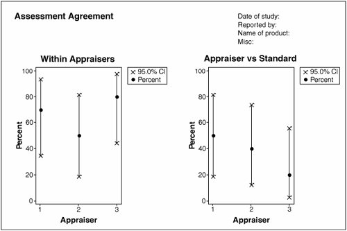
The associated Within Appraiser statistics are shown in Figure 7.26.2. For example, Appraiser 1 agreed with himself in seven out of the ten samples across the two trials. Moving forward, agreement would likely be somewhere between 34.75% and 93.33% (with 95% confidence). To gain a narrower confidence interval, more samples or trials would be required. To be a good, reliable Measurement System, agreement needs to be 90% or better.

Figure 7.26.2. An example of a Within Appraiser Agreement (output from Minitab v14).

Within Appraisers
Assessment Agreement
Appraiser	# Inspected	# Matched	Percent	95% CI
1	10	7	70.00	(34.75, 93.33)
2	10	5	50.00	(18.71, 81.29)
3	10	8	80.00	(44.39, 97.48)
# Matched: Appraiser agrees with him/herself across trials.

The associated Appraiser versus Standard statistics are shown in Figure 7.26.3. For example, Appraiser 1 agreed with the standard in five out of the ten samples. Moving forward, agreement would likely be somewhere between 18.71% and 81.29% (with a 95% degree of confidence). To be a usable Measurement System, agreement needs to be 90% or better, which is clearly not the case here.

Figure 7.26.3. An example of an Appraiser Agreement versus Standard (output from Minitab v14).

Each Appraiser Vs Standard
Assessment Agreement
Appraiser	# Inspected	# Matched	Percent	95% CI
1	10	5	50.00	(18.71, 81.29)
2	10	4	40.00	(12.16, 73.76)
3	10	2	20.00	(2.52, 55.61)
# Matched: Appraiser's assessment across trials agrees with the known standard.

The associated Between Appraiser statistics are shown in Figure 7.26.4. The Appraisers all agreed with one other in four out of the ten samples. Moving forward, agreement would likely be somewhere between 12.16% and 73.76% (with a 95% degree of confidence). To be a reliable Measurement System, agreement needs to be 90% or better, which is clearly not the case here.

Figure 7.26.4. An example of a Between Appraiser Agreement (output from Minitab v14).

Between Appraisers
Assessment Agreement
# Inspected	# Matched	Percent	95% CI
10	4	40.00	(12.16, 73.76)
# Matched: All appraisers' assessments agree with each other.

Another useful statistic in Attribute MSA is Kappa, defined as the proportion of agreement between raters after agreement by chance has been removed. A Kappa value of + 1 means perfect agreement. The general rule is that if Kappa is less than 0.70, then the measurement system needs attention. Table 7.26.1 shows how the statistic should be interpreted.

Table 7.26.1. Interpreting Kappa Results

Kappa	Interpretation
1 to 0.6	Agreement expected by chance
0.6 to 0.7	MarginalSignificant effort required
0.7 to 0.9	GoodImprovement warranted
0.9 to 1.0	Excellent

Figure 7.26.5 shows example Kappa statistics for a light bulb manufacturer's final test Measurement System with five defect categories (Color, Incomplete Coverage, Misaligned Bayonet, Scratched Surface, and Wrinkled Coating). For the defective items, appraisers are required to classify the defective by the most obvious defect. Color and Wrinkle are viable classifications (Kappa > 0.9), but for the rest of the classifications agreement cannot be differentiated from random chance. The p-values here are misleading because they are related to a test of whether the Kappa is (greater than) zero. Just look to the Kappa values for this type of analysis. The overall reliability of the Measurement System is highly questionable because the Kappa for the Overall Test is only 0.52.

Figure 7.26.5. An example of Kappa statistic results for multiple defect categories (output from Minitab v14).

Between Appraisers
Fleiss' Kappa Statistics
Response	Kappa	SE Kappa	Z	P(vs>0)
Color	1.00000	0.0816497	12.2474	0.0000
Incomplete	0.16279	0.0816497	1.9938	0.0231
Misaligned	0.28409	0.0816497	3.4794	0.0003
Scratch	0.17241	0.0816497	2.1116	0.0174
Wrinkle	0.92298	0.0816497	11.3041	0.0000
Overall	0.52072	0.0473565	10.9958	0.0000

After MSA data has been analyzed, the results usually show poor reliability for many Attribute MSAs. This is mainly due to sheer number of ways these types of Measurement Systems can fail:

• Appraiser

  • Visual acuity (or lack of it)

  • General intelligence (more specifically common sense) and comprehension of the goal of the test

  • Individual method of inspection adopted

• Appraisal

  • Defect probability. If this is very high, the appraiser tends to reduce the stringency of the test. The appraiser can become numbed or hypnotized by the sheer monotony of repetition. If this is very low, the appraiser tends to get complacent and tends to see only what he expects to see. This happens in spite of good visual acuity.

  • Fault type. Some defects are far more obvious than others.

  • Number of faults occurring simultaneously. If this is the case, the appraiser has to make the judgment into which category the defective should be classified.

  • Time allowed for inspection.

  • Frequency of rest periods for the appraiser.

  • Illumination of the work area.

  • Inspection station layout. Quite often there isn't enough space to conduct the test effectively or sometimes dedicated space is not provided at all.

  • Time of day and length of time the appraiser has been working.

  • Objectivity and clarity of conformance standards and test instructions.

• Organization and environment.

  • Appraiser training and certification.

  • Peer standards. Defectives are often deemed to reflect badly on coworkers, so the appraiser is constantly under pressure to artificially reduce the defect rates.

  • Management standards. Appraisers often report to someone who is accountable for the volume of shipped product. Reduced volumes reflect poorly on this individual, so they sometimes unconsciously apply pressure on the appraiser to ensure volumes remain high (and defects are allowed to slip by).

  • Knowledge of operator or group producing the item.

  • Proximity of inspectors.

  • Re-inspection versus immediate shipping procedures.

Given all the preceding possibilities for failure it should be apparent why Belts are strongly encouraged to move to Continuous metrics versus Attribute ones. If only Attribute measures are feasible, there are some actions that help improve reliability of the metric, but there really are no guarantees in this area:

• Set very clear Operational Definitions of the metric and defect classifications.

• Train and certify appraisers and revisit this on a regular basis.

• Break up the numbing rhythm with pauses.

  • Introduce greater variety into the job by giving a wider assortment of duties or greater responsibility

  • Arrange for frequent job rotation.

  • Introduce regular rest periods.

• Enhance faults to make them more noticeable.

  • Sense Multipliers Optical magnifiers, sound amplifiers, and other devices to expand the ability of the unaided human to sense the defects/categories.

  • Masks Used to block out the appraisers view of irrelevant characteristics to allow focus on key responsibilities.

  • Templates These are a combination of a gage, a magnifier, and a maskfor example, a cardboard template placed over terminal boards. Holes in the template mate with the projecting terminals and serve as a gage for size. Any extra or misplaced terminal prevents the template from seating properly. Missing terminals become evident because the associated hole is empty.

  • Overlay These are visual aids in the form of transparent sheets on which guidelines or tolerance lines are drawn. Judging size or location of product elements is greatly simplified by such guidelines.

  • Checklists For example, pre-flight checklist on aircraft.

  • Product Redesign In some situations, the product design makes access difficult or places needless complexity or burden on the inspectors. In such cases, product redesign can help reduce inspector errors, as well as operator errors.

  • Error Proofing There are many forms of this, such as redundancy, countdowns, and fail-safe methods (see "Poka Yoke (Mistake Proofing)" in this chapter).

  • Automation Replacement of repetitive inspection with automation that makes no inadvertent errors after the setup is correct and stable. Clearly there are limitations here of cost and the current state of technology.

  • Visual aids Keep an appraiser from having to rely on memory of the standard. The appraiser is provided with a physical standard or photographs against which to make direct comparisons. For example, in the automobile industry, painted plates are prepared exhibiting several scratches of different measured widths and other visual blemishes to define defects in the paint finish.

Attribute Measurement Systems are certainly the most difficult to improve, and it is important to check continually for appraiser understanding. It is generally useful to capture data on a routine basis on the proportion of items erroneously accepted or rejected and applying Statistical Process Control to the Measurement System based on this.