Section 15. Demand Profiling

15. Demand Profiling

Overview

Demand Profiling is simply the application of a Time Series Plot to the Customer demand on a process. It is considered a tool in its own right because

• Understanding demand is so important in any Lean Sigma project

• Interpretation of the plot is the key to success

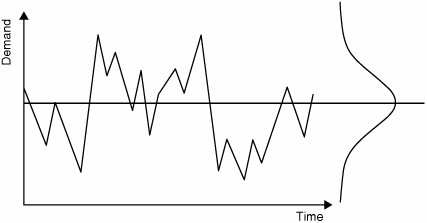
Figure 7.15.1 shows a simple Demand Profile plot. Demand data is captured over time at uniform^[24] time intervals and plotted with an x-axis of Time and a y-axis of Demand. The plot highlights the likely average demand on the process and also the likely variation in demand to which the process has to respond.

^[24] Uniformity isn't imperative but helps greatly in interpretation.

Figure 7.15.1. A simple Demand Profile.

Logistics

As a simple analysis tool this can be applied by the Belt without the rest of the Team, however the data might have to come from multiple sources and often requires Team involvement to collect it. The analysis itself is done entirely in a spreadsheet or statistical package and can be done in a matter of a few minutes after the data is in the correct format.

Initially, data is historical, but after the organization understands the application of the tool, forecast data can also be used.

Roadmap

Step 1.	Identify which entity type or types are to be examined. Demand Profiling represents demand for either one entity type or the sum across a few entity types. If the Team needs to understand the volume and variation across many entity types then it is probably best to look at a Demand Segmentation instead of a Demand Profile.
Step 2.	Identify the time increments. It is necessary to have at least 25 increments of captured demand to have a useful graph. The increments themselves should be meaningful, and it is useful to take the typical replenishment cycle as the driver. For example, if Customers were replenished weekly, then a week would be a reasonable time increment.
Step 3.	Data is collected from the downstream Customer for the entity type for each time increment. The most common mistake is to look to the Process Planning group for when we decided to make the entity, not when it was actually demanded by the Customer. Customer demand rates are typically much smoother than we care to admit, and in fact, their usage rates are even smoother. Internally, we tend to batch entity processing into large lots, which we make on an infrequent basis; so it shows a much higher variation in demand than is actually there. For Demand Profiling, we need to look at demand patterns, not our own planned process patterns.
Step 4.	After the demand data for the entity type across multiple time increments is collected, create the graph similar to the one shown in Figure 7.15.1, taking the time as the x-axis and the volume of demand as the y-axis.

Interpreting the Output

There are some important points to consider when examining the Demand Profile. The purpose of creating the profile was to understand, from historical data, future volume and variation in demand. Using historical data might be misleading; so the first question to consider is whether future usage patterns are expected to be similar to those in the past. It is always useful to study the market and technology changes and factor these into the analysis.

In effect, the Demand Profile is being used as a rudimentary forecasting tool, but rather than using the data to determine how much to generate on a short-term basis, it is used to create a more responsive and capable process.

Demand Profiles can exhibit one or combinations of a multitude of patterns, the most common of which are shown in Figure 7.15.2. See the "Interpreting the Output" section in "Demand Segmentation" in this chapter. Graph A represents a Zone 1 Demand Profile, whereas Graph D represents a Zone 3 Demand Profile.

Figure 7.15.2. Interpreting the Demand Profile.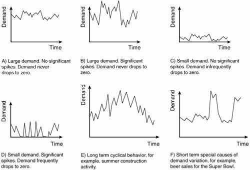

The value that Demand Profiling brings above and beyond Demand Segmentation is that cyclical patterns become visible. Rather than just knowing that there is variation, the Belt obtains an understanding of how the demand is varying. After this is understood, the process can be laid out and resourced accordingly. For example, if there are significant spikes in demand at the end of each day:

• More staff could be used at that point (effectively increasing capacity)

• Inventory could be built ahead of time to serve the demand

• Later staff hours could be used to spread the demand

• Customers could be encouraged not to batch their demand and perhaps spread it to earlier hours, and so on

However, the demand is dealt with from the Demand Profile, without visibility of the variation from the graph, the process is always at its mercy.

Other Options

Although Demand Profiling is simply the use of the graphical tool the Time Series Plot, an obvious extension is the application of statistical analysis to the plot data. Analysis of this form relies on interpolation techniques similar to Regression. Although extremely valuable as an enhanced version of Demand Profiling, it is a difficult and complex subject considered outside the skill set of Black Belts and Green Belts and is considered beyond the scope of this book.

In simple terms the interpolation techniques break down the time series data into its component parts, namely:

• Current Level The mean value at the current time

• Trend The rate of systematic increase (or decrease) in the mean value

• Seasonal Pattern A recurring periodic pattern

• Random Component The portion of behavior that remains unaccounted for after the Current Level, the Trend and the Seasonal Pattern have been identified.^[25]

  ^[25] For further reference see Forecasting: Methods and Applications (3rd Edition) by S. Makridakis, S.C. Wheelwright, and R.J. Hyndman.