Section C. RTY, Defects, Accuracy, Quality, Scrap, and Rework Issues

C. RTY, Defects, Accuracy, Quality, Scrap, and Rework Issues

Overview

Processes are required to generate as high a proportion of perfect entities as possible. Any time a nonperfect entity is generated, capacity is lost, and costs are incurred in lost materials, increased labor, and so forth.

Often rework is disguised under other names, so it is useful to spend some time examining the process to understand exactly how cost is being incurred.

Examples

Industrial. Reworking of downgrade product (blending off), downgrading product, line scrap, and material loss
Healthcare. Patient handoff (incompleteness of information), medications delivery/administration accuracy, clinical defects such as Ventilator-Acquired Pneumonia
Service/Transactional. Billing accuracy, order accuracy

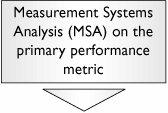
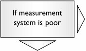
Measuring Performance

In considering quality, typical primary measures would comprise

Rolled Throughput Yield (RTY) or First Time Right measured as
- The percentage of entities that make it all the way through the process Right First Time, every step along the way. This is not to be confused with the final Yield of the process, which typically is inflated with rework throughout the process. The RTY is commonly much lower than understood by the business.
Primary Performance Metric(s)
- The process has a performance characteristic(s) for the entities it generates that is being measured against a specification (e.g., a dimension, strength, or other physical/chemical characteristic).

RTY is a conformance metric in that it represents the percentage of occurrences conforming to a specification on a performance metric. It is often better to proceed through the roadmap using the performance characteristic(s) itself as the primary metric, rather than a conformance metric such as RTY. If all else fails, use RTY as the primary metric.

Tool Approach

If not already done in a previous step, commence the roadmap with

More than likely, this will involve a detailed measurement system reliability study (a Gage R&R study for continuous data, or an Attribute MSA/Kappa study for attribute data), rather than just a simple validation. An MSA will be required for each performance characteristic for the entity (e.g., strength and water absorption requires two separate MSAs to be completed). See "MSAValidity," "MSAContinuous," and "MSAAttribute" in Chapter 7, "Tools."

Sometimes the entire problem comes down to an issue with the measurement system. If the MSA conducted previously shows a high % R&R or P/T ratio, move to Section L in this chapter to mend the System.

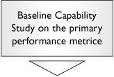
After the measurement system has been validated, perform

For attribute data, this will simply be RTY, Defects Per Unit (DPU), or Defects Per Million Opportunities (DPMO). At least 100 data points will be required if the defect rate is high (>5%), and more if the defect rate is lower. For more details see "CapabilityAttribute" in Chapter 7.

For continuous data conduct, a full Capability Study to calculate C_p and C_pk will be needed. At least 25 data points will be required. For more details see "CapabilityContinuous" in Chapter 7.

For both data types, data must be captured over a period long enough for typical process noises to have an effect. For example, if there are monthly fluctuations, data needs to be available across two months or more. Capture one to two weeks' worth of data to get a rough estimate of capability, but continue down the roadmap in parallel while continuing to collect the capability data.

At this point, the problem has been resolved in that the measurement system was the problem (or it's a remote possibility that previous Capability Studies were flawed), in which case see the Control tools in Chapter 5, "ControlTools Used at the End of All Projects." If not, proceed down the roadmap in this section.

The roadmap to a solution from this point forward relies on the equation Y=f(X₁, X₂,..., X_n), where the Y is the Primary Performance characteristic(s):

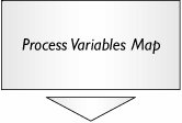
[Pages 32 - 33]

	This tool will identify all input variables (Xs) that cause changes in the Primary Performance Metric(s) (Ys), otherwise known as output variables. Any obviously problematic uncontrolled Xs should be added directly to the Process Failure Mode and Effects Analysis (FMEA).
	The Xs generated by the Process Variables Map are transferred directly into the C&E Matrix. The Team uses its existing knowledge of the process through the matrix to eliminate the Xs that don't affect the Ys. If the process has many steps, consider a two-phase C&E Matrix as follows: Phase 1List the process steps (not the Xs) as the items to be prioritized in the C&E Matrix. Reduce the number of steps based on the effect of the steps as a whole on the Ys. Phase 2For the reduced number of steps, enter the Xs for only those steps into a second C&E Matrix and use this matrix to reduce the Xs to a manageable number. Phase 3Make a quick check on Xs from the steps eliminated in Phase 1 to ensure that no obviously vital Xs have been eliminated.
	The reduced set of Xs from the C&E Matrix are entered into the FMEA. This tool will narrow them down further, and generate a set of action items to eliminate or reduce high-risk process areas. This is as far as the Team can proceed without detailed process data on the Xs. The FMEA is the primary tool to manage the obvious Quick Hit changes to the process that will eliminate special causes of variation. At this point, the problem may be reduced enough to proceed to the Control tools in Chapter 5. If not, continue down this roadmap.
	The reduced set of Xs from the FMEA is carried over into this array of tools along with the major Ys from the Process Variables Map. Statistical tools applied to actual process data will help answer the following questions: Which Xs (probably) affect the Ys? Which Xs (probably) don't affect the Ys? How much variation in the Ys is explained by the Xs identified? The word probably is used because this is statistics, and hence there is a degree of confidence associated with every inference made. This tool will narrow the Xs down to the few key Xs that (probably) drive most of the variation on the Ys. In service/administrative/transactional processes, it is usually possible to move straight from this point to the Control tools in Chapter 5 without conducting any Designed Experiments unless some kind of (computer) simulation of the process can be made. For more details on Designed Experiments see "DOEIntroduction" in Chapter 7.
	If there are still a large number of Xs (6 or more) left after the Multi-Vari Study, it is best to reduce that set using a Fractional Factorial DOE. This tool will only identify the key Xs and should not be used to investigate interactions or to optimize the process.
	The reduced set of Xs from the Screening Design is more deeply understood using a Full Factorial Design. This tool will help us determine the final reduced set of Xs to be controlled in the process, along with any interactions between those Xs. Another output will be the amount of variability explained by these Xs. It is possible at this point that the process is understood deeply enough and the results are good enough that no further optimization is required. If this is the case, proceed to the Control tools in Chapter 5; if not, continue down the roadmap here.
	In a small number of instances, it might be appropriate to use Response Surface Methodology (RSM) (or simply Regression if we have narrowed down to just one X) to optimize the level of the Xs to maximize performance of the Ys. After the best levels for the critical Xs have been determined, proceed to the Control tools in Chapter 5.