52. t-Test1-Sample Overview The 1-Sample t-Test is used to compare a sample mean against a specific target value. For example, a Team might need to determine if an operator is taking a certain amount of time to perform a task. The target value would be the nominal task time, and a data sample would be taken of, for example, 25 points to make the judgment. The result is the likelihood that the average operator task time (as work continues thenceforth) is the same as the nominal value. Thus, a sample of data points (lower curve) is taken from the process (the population of all data points, upper curve), as shown in Figure 7.52.1. From the characteristics of the sample (mean standard deviation s, and sample size n), an inference is made on the location of the population mean  relative to the target value. The result would be a degree of confidence (a p-value) that the sample came from a population with mean μ the same as the target. relative to the target value. The result would be a degree of confidence (a p-value) that the sample came from a population with mean μ the same as the target. Figure 7.52.1. Graphical representation of a 1-Sample t-Test. 
Roadmap The roadmap of the test analysis itself is shown graphically in Figure 7.52.2. Figure 7.52.2. 1-Sample t-Test Roadmap.[89] 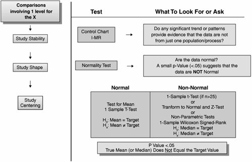
[89] Roadmap adapted from SBTI's Process Improvement Methodology training material.
Step 1. | Identify the metric and target value. Analysis of this kind should be done in the Analyze Phase at the earliest, so the metric should be well defined and understood at this point (see "KPOVs and Data" in this chapter).
| | | Step 2. | Determine the sample size. This can be as simple as taking the suggested 25 data points or using a sample size calculator in a statistical package. These rely on an equation relating the sample size to
The standard deviation (the spread of the data). This would have to be approximated from historical data. The required power of the test (the likelihood of the test seeing a difference between the mean and the target value if there truly was one). This is usually set at 0.8 or 80%. The power is actually (1 β), where β is the likelihood of giving a false negative and might need to be entered as a β of 0.2 or 20%. The size of the difference σ between the mean and the target value that is desired to be detected (i.e., the size of deviation from the target that would lead the Team to say that the two values were different). The alpha level for the test (the likelihood of the test giving a false positive) usually set at 0.05 or 5% and represents the cutoff for the p-value (remember if p is low, H0 must go). Whether the test is one-tailed or two-tailed see "Other Options" in this section.
| | | Step 3. | Collect the sample following the rules of good experimentation.
| Step 4. | Examine stability of the sample data using a Control Chart, typically an Individuals and Moving Range Chart (I-MR). A Control Chart identifies whether the process is stable, that is having
This is important because if the process is moving around, it is impossible to sensibly make the call as to whether it is on target or not.
| Step 5. | Examine normality of the sample data using a Normality Test. This is important because the statistical test in Step 6 relies on it, but in simple terms if the sample curve in Figure 7.52.1 were a strange shape it would be difficult to determine if the middle of it were off target. In fact if the data becomes skewed, then the mean is probably not the best measure of center (a t-Test is a mean-based test), and a median-based test is probably better. The longer tail on the right of the curve drags the mean to the right; however, the median tends to remain constant, see Figure 7.52.3. Medians-based tests can, in theory, be used for everything as a more robust test, but they are less powerful than their means-based counterparts, and, hence, the desire to go with the mean.
Figure 7.52.3. Measures of Center. 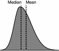
| | | Step 6. | Perform the 1-Sample t-Test if the sample data was normal. The hypotheses in this case are
If the data were non-normal, then as per Figure 7.52.2:
Continue unabated with the 1-Sample t-Test if the sample size is large enough (>25) Transform the data and perform the analysis using a 1-Sample Z-Test Perform the median-based equivalent test, a Wilcoxon Test (if the data is symmetrical) or a Signed-Rank Test if not
The last option sounds complicated, but the medians tests look identical in form to the means test and both return the key item, a p-value (the p-values are unlikely to be the same though).
|
Interpreting the Output The 1-Sample t-Test[90] compares the sample characteristics (mean standard deviation s, and sample size n) to a reference distribution, the t-distribution, to determine whether the sample indicates that the population is statistically different from the target or not. Amongst other things, it returns a p-value; the likelihood that for the sample a difference from a target this large can have occurred purely by random chance even if the population were on target. [90] The technical details of a t-Test are covered in most statistics textbooks; Statistics for Management and Economics by Keller and Warrack makes it understandable to non-statisticians.
Based on the t-Test and the p-values, statements can be generally formed as follows: Based on the data, I can say that there is a statistically significant difference and there is a (p-value) chance that I am wrong Or based on the data, I can say that there is an important effect and there is a (p-value) chance the result is just due to chance
Output from a 1-Sample t-Test is shown in Figure 7.52.4. Figure 7.52.4. Test results for a comparison of a sample of Bob's performance data versus a target value of 25.One-Sample T: Bob | | | | Test of mu = 25 vs not = 25 | | | | Variable | N | Mean | StDev | SE Mean | 95% CI | T | P | Bob | 30 | 24.8482 | 0.8693 | 0.1587 | (24.5236, 25.1728) | 0.96 | 0.347 |
From the example results They are based on hypotheses μ = 25 (H0) versus μ  25 (Ha) 25 (Ha) The mean of the sample was 24.8482 The standard deviation of the sample was 0.8693 There is a 95% likelihood that the mean of the population lies between 24.5236 and 25.1728 The mean of the sample lies 0.96 Standard Errors (0.1587) below the target (hence the minus sign) The likelihood of seeing a sample mean  this far from the target value (if the population were actually perfectly on target) is 34.7% (p-value), which is above 0.05; thus, a conclusion that Bobs performance cannot be differentiated from target given the sample data. this far from the target value (if the population were actually perfectly on target) is 34.7% (p-value), which is above 0.05; thus, a conclusion that Bobs performance cannot be differentiated from target given the sample data.
Other Options The test described previously has hypotheses defined as Therefore, this test is known as a two-tailed test, because (by the " " in Ha) it is not known whether the mean is above or below target. Therefore, the test needs to cover both sides (tails). " in Ha) it is not known whether the mean is above or below target. Therefore, the test needs to cover both sides (tails). A one-tailed test, on the other hand, is used when it can be stated up front whether the mean is above target or below target. The hypotheses in this case would either be or A one-tailed test (greater than or less than) can detect a smaller difference between the mean and the target value than a two-tailed test[91] (not equal to). Given the choice, go with the one-tailed test if there is data to show which side of the target value the mean is sitting. [91] A detailed explanation of the reason for this can be found in most statistics textbooks; Statistics for Management and Economics by Keller and Warrack is useful here.
|