7.3 Nonlinear Predictive Techniques

Linear predictive methods exploit the wideband nature of the useful data signal to suppress the interference. In doing so, they are exploiting only the spectral structure of the spread data signal, not its further structure. These techniques can be improved upon in this application by exploiting such further structure of the useful data signal as it manifests itself in the sampled observations (7.5). In particular, on examining (7.1), (7.2), (7.3), and (7.5), we see that for the single- user case (i.e., K = 1), the discrete-time data signal { c _n } takes on values of only . Although linear prediction would be optimal in the model of (7.5) in the case in which all signals are Gaussian, this binary-valued direct-sequence data signal { c _n } is highly non-Gaussian. So, even if the NBI and background noise are assumed to be Gaussian, the optimal filter for performing the required prediction will, in general, be nonlinear (e.g., [377]). This non-Gaussian structure of direct-sequence signals can be exploited to obtain nonlinear filters that exhibit significantly better suppression of narrowband interference than do linear filters under conditions where this non-Gaussian-ness is of sufficient import. In the following paragraphs we elaborate on this idea, which was introduced in [522] and explored further in [133, 376, 387, 425, 535 “538].

Consider again the state-space model of (7.10) “(7.11). The Kalman “Bucy estimator discussed above is the best linear predictor of r _n from its past values. If the observation noise { v _n } of (7.12) were a Gaussian process, this filter would also give the global MMSE (or conditional mean) prediction of the received signal (and hence of the interference). However, since { v _n } is not Gaussian but rather is the sum of two independent random variables , one of which is Gaussian and the other of which is binary ( ), its probability density is the weighted sum of two Gaussian densities . In this case, the exact conditional mean estimator can be shown to have a complexity that increases exponentially in time [452], which renders it unsuitable for practical implementation.

7.3.1 ACM Filter

In [309], Masreliez proposed an approximate conditional mean (ACM) filter for estimating the state of a linear system with Gaussian state noise and non-Gaussian measurement noise. In particular, Masreliez proposed that some, but not all, of the Gaussian assumptions used in derivation of the Kalman filter be retained in defining a nonlinearly recursively updated filter. He retained a Gaussian distribution for the conditional mean, although it is not a consequence of the probability densities of the system (as is the case for Gaussian observation noise), hence the name approximate conditional mean that is applied to this filter. In [133, 387, 522] this ACM filter was developed for the model (7.10) “(7.11). To describe this filter, first denote the prediction residual by

Equation 7.34

This filter operates just as that of (7.13) “(7.17), except that the measurement update equation (7.14) is replaced with

Equation 7.35

and the update equation (7.16) is replaced with

Equation 7.36

The terms g _n and G _n are nonlinearities arising from the non-Gaussian distribution of the observation noise and are given by

Equation 7.37

Equation 7.38

where we have used the notation , and p ( ) denotes the measurement prediction density. The measurement updates reduce to the standard equations for the Kalman “Bucy filter when the observation noise is Gaussian.

For the single-user system, the density of the observation noise in (7.12) is given by the following Gaussian mixture:

Equation 7.39

Let be the variance of the innovation (or residual) signal in (7.34):

Equation 7.40

we can then write the functions g _n and G _n in this case as

Equation 7.41

Equation 7.42

The ACM filter is thus seen to have a structure similar to that of the standard Kalman “Bucy filter. The time updates (7.13) and (7.15) are identical to those in the Kalman “Bucy filter. The measurement updates (7.35) and (7.36) involve correcting the predicted value by a nonlinear function of the prediction residual _n . This correction essentially acts like a soft-decision feedback to suppress the spread-spectrum signal from the measurements. That is, it corrects the measurement by a factor in the range [ ] that estimates the spread-spectrum signal. When the filter is performing well, the variance term in the denominator of tanh( ·) is low. This means that the argument of tanh( ·) is larger, driving tanh( ·) into a region where it behaves like the sign( ·) function, and thus estimates the spread-spectrum signal to be if the residual signal _n is positive and if the residual is negative. On the other hand, when the filter is not making good estimates, the variance is high and tanh( ·) is in a linear region of operation. In this region, the filter hedges its bet on the accuracy of sign( _n ) as an estimate of the spread-spectrum signal. Here the filter behaves essentially like the (linear) Kalman filter. The ACM-filter-based NBI suppression algorithm based on the state-space model (7.10) “(7.11) is summarized as follows .

Algorithm 7.3: [ACM-filter-based NBI suppression] At time i, N received samples {r _iN , r _iN+1 , ..., r _iN+N-1 } are obtained at the chip-matched filter output (7.5) .

• For n = iN, iN + 1, ..., iN + N - 1 perform the following steps:

  Equation 7.43

  

  
  

  Equation 7.44

  

  
  

  Equation 7.45

  

  
  

  Equation 7.46

  

  
  

  Equation 7.47

  

  
  

  Equation 7.48

  

  
  

  where g _n and G _n are defined in (7.41) and (7.42), respectively .

• Detect the ith bit b ₁ [ i ] according to

  Equation 7.49

  

  
  

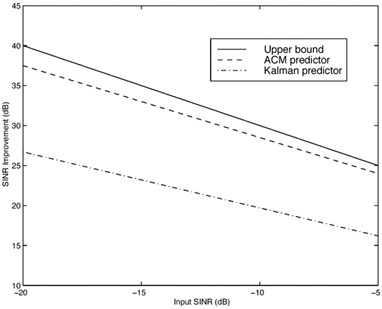
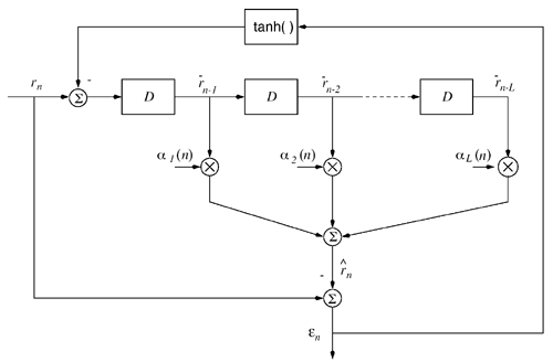
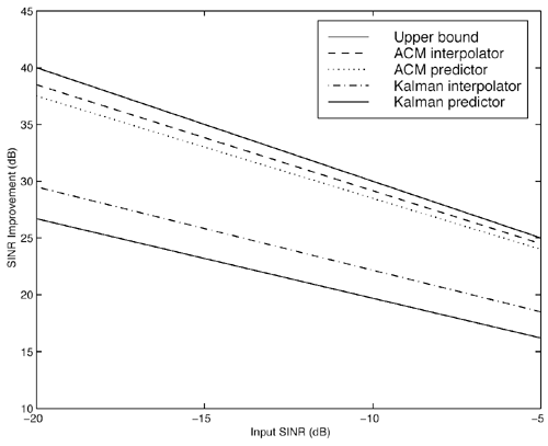
Simulation Examples

When the interference is modeled as a first-order autoregressive process, which does not have a very sharply peaked spectrum, the performance of the ACM filter does not seem to be appreciably better than that of the Kalman “Bucy filter. However, when the spectrum of the interference is made to be more sharply peaked by increasing the order of the autoregression, the ACM filter is found to give significant performance gains over the Kalman filter. Simulations were run for a second-order AR interferer with both poles at 0.99:

where { e _n } is an i.i.d. Gaussian sequence. The ambient noise power is held constant at s ² = 0.01, while the total of noise plus interference power varies from 5 to 20 dB (all relative to a unity power spread-spectrum signal). In comparing filtering methods, the figure of merit is the ratio of SINR at the output of filtering to the SINR at the input, which reduces to

where _n is defined as in (7.34). The results from the Kalman and ACM predictors are shown in Fig. 7.5. The filters were run for 1500 points. The results reflect the last 500 points, and the values given represent averages over 4000 independent simulations.

Figure 7.5. Performance of the Kalman filter “ and ACM filter “based NBI suppression methods.

To stress the effectiveness against the narrowband interferer (versus the background noise), the solid line in Fig. 7.5 gives an upper bound on SNR improvement, assuming that the narrowband interference is predicted with noiseless accuracy. This is calculated by setting equal to the power of the AWGN driving the AR process (i.e., the unpredictable portion of the interference). Note that the SINR improvement due to using the ACM filter is quite substantial and is very near the theoretical bound.

7.3.2 Adaptive Nonlinear Predictor

It is seen that in the ACM filter, the predicted value of the state is obtained as a linear function of the previous estimate modified by a nonlinear function of the prediction error. We now use the same approach to modify the adaptive linear predictive filter described in Section 7.2.2. This technique was first developed in [387, 522]. To show the influence of the prediction error explicitly, using (7.34) we rewrite (7.25) as

Equation 7.50

We make the assumption, similar to that made in the derivation of the ACM filter, that the prediction residual _n is the sum of a Gaussian random variable and a binary random variable. If the variance of the Gaussian random variable is , the nonlinear transformation appearing in the ACM filter can be written as

Equation 7.51

By transforming the prediction error in (7.50) using the nonlinearity above, we get a nonlinear transversal filter for the prediction of r _n , namely,

Equation 7.52

where is given by

Equation 7.53

The structure of this filter is shown in Fig. 7.6. To implement the filter of (7.52), an estimate of the parameter and an algorithm for updating the tap weights must be obtained. A useful estimate for is , where D _n is a sample estimate of the prediction error variance [e.g., ]. On the other hand, the tap-weight vector can be updated according to the modified LMS algorithm

Figure 7.6. Tapped-delay-line nonlinear predictor.

Equation 7.54

where and p _n is given by (7.28). Note that the nonlinear prediction given by (7.52) is recursive in the sense that the prediction depends explicitly on the previous predicted values as well as on the previous input to the filter. This is in contrast to the linear prediction of (7.25), which depends explicitly only on the previous inputs to the filter, although it depends on the previous outputs implicitly through their influence on the tap-weight updates. The nonlinear prediction-based NBI suppression algorithm is summarized as follows.

Algorithm 7.4: [LMS nonlinear prediction-based NBI suppression] At time i, N received samples {r _iN , r _iN+1 , ..., r _iN+N-1 } are obtained at the chip-matched filter output (7.5) .

• For n = iN, iN + 1, ..., iN + N - 1 perform the following steps:

  Equation 7.55

  

  
  

  Equation 7.56

  

  
  

  Equation 7.57

  

  
  

  Equation 7.58

  

  
  

• Detect the ith bit b ₁ [ i ] according to

  Equation 7.59

  

  
  

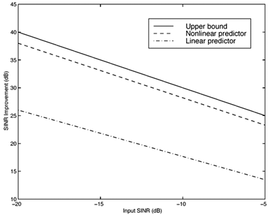
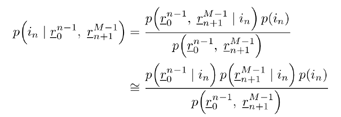
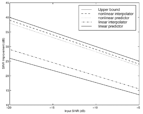
It is interesting to note that the predictor (7.52) can be viewed as a generalization of both linear and hard- decision-feedback (see, e.g., [107, 108, 254]) adaptive predictors, in which we use our knowledge of the prediction error statistics to make a soft decision about the binary signal, which is then fed back to the predictor. As noted above, introduction of this nonlinearity improves the prediction performance over the linear version. As discussed in [387], softening of this feedback nonlinearity improves the convergence properties of the adaptation over the use of hard-decision feedback.

Simulation Examples

To assess the nonlinear adaptive NBI suppression algorithm above, simulations were performed on the AR model for interference given in Section 7.2. The results are shown in Fig. 7.7. It is seen that, as in the case where the interference statistics are known, the nonlinear adaptive NBI suppression method significantly outperforms its linear counterpart .

Figure 7.7. Performance of adaptive linear predictor “ and adaptive nonlinear predictor “based NBI suppression methods.

7.3.3 Nonlinear Interpolating Filters

ACM Interpolator

Nonlinear interpolative interference suppression filters have been developed in [425]. We next derive the interpolating ACM filter. We consider the density of the current state conditioned on previous and following states. We have

Equation 7.60

Equation 7.61

where in (7.60) we made the approximation that, conditioned on i _n , and are independent. The second term in (7.61) is independent of i _n . If it is assumed (analogously to what is done in the ACM filter) that the two densities in the numerator of the first term in (7.61) are Gaussian, the interpolated estimate is also Gaussian. Therefore, if we assume that the densities are (where f indicates the forward prediction and b indicates the backward prediction)

the interpolated estimate is still Gaussian:

Equation 7.62

with

Equation 7.63

Equation 7.64

While the mean and variance of the interpolated estimate at each sample n can be computed via the equations above, recall that the forward and backward means and variances are determined by the nonlinear ACM filter recursions.

Simulation Examples

The equations above can be used for both the linear Kalman filter and the ACM filter to generate interpolative predictions from the forward and backward predicted estimates. As in the ACM prediction filter, we have approximated the conditional densities as being Gaussian, although the observation noise is not Gaussian. The filters are run forward on a block of data and then backward on the same data. The two results are combined to form the interpolated prediction via (7.63) “(7.64).

Simulations were run on the same AR model for interference as that given in Section 7.2. Figure 7.8 gives results for interpolative filtering over predictive filtering for the known statistics case. The filters were run forward and backward for all 1500 points in the block. Interpolator SINR gain was calculated over the middle 500 points (when both forward and backward predictors were in steady state).

Figure 7.8. Performance of Kalman interpolator “ and ACM interpolator “based NBI suppression methods.

Adaptive Nonlinear Block Interpolator

Recall that the ACM predictor uses the interference prediction at time n , , to generate a prediction of the observation less the spread spectrum signal . This estimate is used in subsequent samples to generate new interference predictions. Since the estimates of are not available for > 0 at time n (i.e., samples that occur after the current one), the ACM filter cannot be cast directly in the interpolator structure. However, an approach similar to the one for the known-statistics ACM interpolator can be used. In this approach the data are segmented into blocks and run through a forward filter of length L to give predictions and . The same data are run through a backward adaptive ACM filter with a separate tap-weight vector, also of length L , to generate estimates and . After these calculations are made for the entire block, the data are combined to form an interpolated prediction according to

Equation 7.65

Equation 7.66

The next block of data follows the same procedure. However, when the next block is initialized , the previous tap weights are used to start the forward predictor, and the interpolated predictions { } are used to initialize the forward prediction. This "head start" on the adaptation can only take place in the forward direction. We do not have any information on the following block of data to give us insight into the backward prediction. Therefore, the backward prediction is less reliable than the forward prediction. To compensate for this effect, consecutive blocks are overlapped , with the overlap being used to allow the backward predictor some startup time to begin good predictions of the spread-spectrum signal [381, 425].

Simulation Examples

Results for the same simulation when the statistics are unknown are given in Fig. 7.9. The adaptive interpolator had a block length of 250 samples, with 100 samples being overlapped. That is, for each block of 250 samples, 150 interpolated estimates were made. For the case of known statistics, the ACM predictor already performs well, and there is little margin for improvement via use of an interpolator. The adaptive filter shows greater margin for improvement, on which the interpolator capitalizes. However, in either case, the interpolator does offer improved phase characteristics and some performance gain at the cost of additional complexity and a delay in processing.

Figure 7.9. Performance of linear interpolator “ and nonlinear interpolator “based NBI suppression methods.

A number of further results have been developed using and expanding the ideas discussed above. For example, performance analysis methods have been developed for both predictive [537] and interpolative [538] nonlinear suppression filters. Predictive filters for the further situation in which the ambient noise { N ( t )} has impulsive components have been developed in [133]. The multiuser case, in which K > 1, has been considered in [425]. Further results can be found in [11, 15, 238, 535, 536].

7.3.4 HMM-Based Methods

In the prediction-based methods discussed above, the narrowband interference environment is assumed to be stationary or, at worst, slowly varying. In some applications, however, the interference environment is dynamic in that narrowband interferers enter and leave the channel at random and at arbitrary frequencies within the spread bandwidth. An example of such an application arises in the littoral sonobuoy arrays mentioned in Section 7.1, in which shore-based commercial VHF traffic, such as dispatch traffic, appears throughout the spread bandwidth in a very bursty fashion. A similar phenomenon arises when the direct-sequence system coexists with a frequency- hopping system, which happens, for example, when wireless LANs and Bluetooth systems operate in the same location. A difficulty with use of adaptive prediction filters of the type noted above is that when an interferer suddenly drops out of the channel, the " notch " that the adaptation algorithm created to suppress it will persist for some time after the signal leaves the channel. This is because, while the energy of the narrowband source drives the adaptation algorithms to suppress an interferer when it enters the channel, there is no counterbalancing energy to drive the adaptation algorithm back to normalcy when an interferer exits the channel. That is, there is an asymmetry between what happens when an interferer enters the channel and what happens when an interferer exits the channel. If interferers enter and exit randomly across a wide band , this asymmetry will cause the appearance of notches across a large fraction of the spread bandwidth, which will result in a significantly degraded signal of interest. Thus, a more sophisticated approach is needed for such cases. One such approach, described in [67], is based on a hidden-Markov model (HMM) for the process controlling the exit and entry of NBIs in the channel. An HMM filter is then used to detect the subchannels that are hit by interferers, and a suppression filter is placed in each such subchannel as it is hit. When an exit is detected in a subchannel, the suppression filter is removed from that subchannel. Related ideas for interference suppression based on HMMs and other "hidden data" models have been explored in [219, 238, 355, 375].