DATA MINING SYSTEM LERS

Chapter VI - Data Mining Based on Rough Sets
Data Mining: Opportunities and Challenges
by John Wang (ed)
Idea Group Publishing 2003

	Brought to you by Team-Fly

The rule induction system, called Learning from Examples using Rough Sets (LERS), was developed at the University of Kansas. The first implementation of LERS was done in Franz Lisp in 1988.

The current version of LERS, implemented in C and C++, contains a variety of data-mining tools. LERS is equipped with the set of discretization algorithms to deal with numerical attributes. Discretization is an art rather than a science, so many methods should be tried for a specific data set. Similarly, a variety of methods may help to handle missing attribute values. On the other hand, LERS has a unique way to work with inconsistent data, following rough set theory. If a data set is inconsistent, LERS will always compute lower and upper approximations for every concept, and then will compute certain and possible rules, respectively.

The user of the LERS system may use four main methods of rule induction: two methods of machine learning from examples (called LEM1 and LEM2; LEM stands for Learning from Examples Module) and two methods of knowledge acquisition (called All Global Coverings and All Rules). Two of these methods are global (LEM1 and All Global Coverings); the remaining two are local (LEM2 and All Rules).

Input data file is presented to LERS in the form illustrated in Table 5. In this table, the first line (any line does not need to be one physical line it may contain a few physical lines) contains declaration of variables: a stands for an attribute, d for decision, x means "ignore this variable." The list of these symbols starts with "<" and ends with ">". The second line contains declaration of the names of all variables, attributes, and decisions, surrounded by brackets. The following lines contain values of all variables.

Table 5: Input data for LERS

< a a a a d >
[Home	Boat	Credit_Card	Age	Loan_Application]
expensive	no	yes	old	approved
middle	yes	no	old	rejected
expensive	yes	no	old	approved
cheap	yes	yes	young	rejected
middle	yes	yes	middle	approved
middle	no	no	old	rejected
middle	no	yes	young	approved
expensive	no	no	young	rejected
expensive	no	no	young	approved

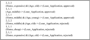
LEM1 Single Global Covering

In this option, LERS may or may not take into account priorities associated with attributes and provided by the user. For example, in a medical domain, some tests (attributes) may be dangerous for a patient. Also, some tests may be very expensive, while at the same time the same decision may be made using less expensive tests. LERS computes a single global covering using the following algorithm:

Algorithm SINGLE GLOBAL COVERING Input: A decision table with set A of all attributes and decision d; Output: a single global covering R; begin    compute partition U/IND(A);    P : = A;    R : =  ;    if U/IND(A) ≤ U/IND({d})       then          begin             for each attribute a in A do                begin                   Q : = P - {a};                   compute partition U/IND(Q);                   if U/IND(Q) ≤ U/IND({d}) then P : = Q                end {for}             R : = P          end {then} end {algorithm}. 

The above algorithm is heuristic, and there is no guarantee that the computed global covering is the simplest. However, the problem of looking for all global coverings in order to select the best one is of exponential complexity in the worst case. LERS computes all global coverings in another option, described below. The option of computing of all global coverings is feasible for small input data files and when it is required to compute as many rules as possible. After computing a single global covering, LEM1 computes rules directly from the covering using a technique called dropping conditions (i.e., simplifying rules).

For data from Table 1 (this table is consistent), the rule set computed by LEM1 is presented in Figure 3. CLOSE UP THIS SPACE. Note that rules computed by LERS are preceded by three numbers: specificity, strength, and the total number of training cases matching the left-hand side of the rule. These parameters are defined previously.

Figure 3: Rule set computed by LEM1 from consistent data.

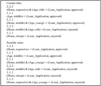
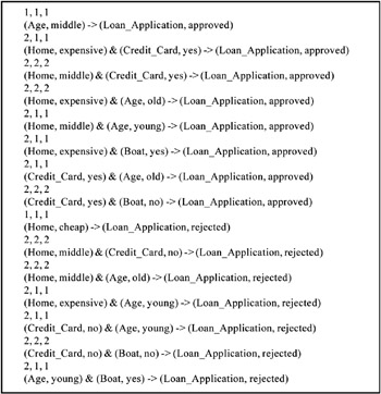
The LEM1 applied to data from Table 2 (this table is inconsistent) computed the rule set presented in Figure 4.

Figure 4: Rule set computed by LEM1 from inconsistent data.

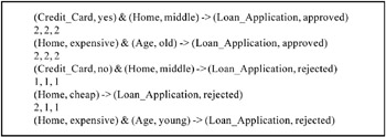
LEM2 Single Local Covering

Like in LEM1 (single global covering option of LERS), in the option LEM2 (single local covering), the user may take into account attribute priorities. In LEM2 option, LERS uses the following algorithm for computing a single local covering:

Algorithm SINGLE LOCAL COVERING Input: A decision table with a set A of all attributes and concept B; Output: A single local covering T of concept B; begin    G : = B;    T : =  ;    while G '''        begin       T : =  ;       T(G) : = {(a, v) | a ε A, v is a value of a, [(a, v)] ∩ G ≠  };       while T =   or [T] ⊊ B       begin          select a pair (a, v) ε T(G) with the highest attribute priority, if a          tie occurs, select a pair (a, v) ε T(G) such that |[(a, v)] ∩ G| is          maximum; if another tie occurs, select a pair (a, v) ε T(G) with          the smallest cardinality of [(a, v)]; if a further tie occurs, select          first pair;          T : = T ∪ {(a, v)};          G : = [(a, v)] ∩ G;          T(G) : = {(a, v) | [(a, v)] ∩ G ≠  };          T(G) : = T(G) - T;       end {while}    for each (a, v) in T do       if [T - {(a, v)}] ⊆ B then T : = T - {(a, v)};          T : = T ∪ {T};          G : = B - ∪ [T];                   T ε T    end {while};    for each T in T do          if ∪ [S] = B then T : = T - {T};              S ε T-{T} end {algorithm}. 

Like the LEM1 option, the above algorithm is heuristic. The choice of used criteria was found as a result of many experiments (Grzymala-Busse & Werbrouck, 1998). Rules are eventually computed directly from the local covering, no further simplification (as in LEM1) is required. For Table 1, LEM2 computed the rule set presented in Figure 5.

Figure 5: Rule set computed by LEM 2.2, 2, 2.

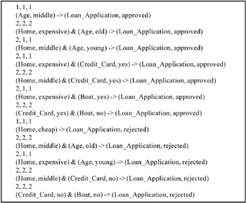
All Global Coverings

The All Global Coverings option of LERS represents a knowledge acquisition approach to rule induction. LERS attempts to compute all global coverings, and then all minimal rules are computed by dropping conditions. The following algorithm is used:

 Algorithm ALL GLOBAL COVERINGS Input: A decision table with set A of all attributes and decision d; Output: the set R of all global coverings of {d}; begin    R : =  ;    for each attribute a in A do       compute partition U/IND({a});    k : = 1;    while k ≤ |A| do       begin          for each subset P of the set A with |P| = k do             if (P is not a superset of any member of R)                   and (∏ U/IND({a}) ≤ U/IND({d})                      a ε P                then add P to R,          k : = k+1       end {while}    end {algorithm}. 

As we observed before, the time complexity for the problem of determining all global coverings (in the worst case) is exponential. However, there are cases when it is necessary to compute rules from all global coverings (Grzymala-Busse & Grzymala-Busse, 1994). Hence, the user has an option to fix the value of a LERS parameter, reducing in this fashion the size of global coverings (due to this restriction, only global coverings of the size not exceeding this number are computed).

For example, from Table 1, the rule set computed by All Global Coverings option of LERS is presented in Figure 6.

Figure 6: Rule set computed by All Global Coverings option of LERS.

All Rules

Yet another knowledge acquisition option of LERS is called All Rules. It is the oldest component of LERS, introduced at the very beginning in 1988. The name is justified by the way LERS works when this option is invoked: all rules that can be computed from the decision table are computed, all in their simplest form. The algorithm takes each example from the decision table and computes all potential rules (in their simplest form) that will cover the example and not cover any example from other concepts. Duplicate rules are deleted. For Table 1, this option computed the rule et presented in Figure 7.

Figure 7: Rule set computed by All Rules option of LERS.

Classification

In LERS, the first classification system to classify unseen cases using a rule set computed from training cases was used in the system, Expert System for Environmental Protection (ESEP). This classification system was much improved in 1994 by using a modified version of the bucket brigade algorithm (Booker et al., 1990; Holland et al., 1986). In this approach, the decision to which concept an example belongs is made using three factors: strength, specificity, and support. They are defined as follows: Strength factor is a measure of how well the rule has performed during training. Specificity is the total number of attribute-value pairs on the left-hand side of the rule. The third factor, support, is related to a concept and is defined as the sum of scores of all matching rules from the concept. The concept getting the largest support wins the contest.

In LERS, the strength factor is adjusted to be the strength of a rule, i.e., the total number of examples correctly classified by the rule during training. The concept C for which support, i.e., the following expression

is the largest is a winner, and the example is classified as being a member of C.

If an example is not completely matched by any rule, some classification systems use partial matching. System AQ15, during partial matching, uses a probabilistic sum of all measures of fit for rules (Michalski et al., 1986).

In the original bucket brigade algorithm, partial matching is not considered a viable alternative of complete matching. Bucket brigade algorithm depends instead on default hierarchy (Holland et al., 1986).

In LERS, partial matching does not rely on the user's input. If complete matching is impossible, all partially matching rules are identified. These are rules with at least one attribute-value pair matching the corresponding attribute-value pair of an example.

For any partially matching rule R, the additional factor, called Matching factor (R), is computed. Matching factor(R) is defined as the ratio of the number of matched attribute-value pairs of a rule R with the case to the total number of attribute-value pairs of the rule R. In partial matching, the concept C for which the following expression is the largest

is the winner, and the example is classified as being a member of C.

LERS assigns three numbers to each rule: specificity, strength, and the total number of training cases matching the left-hand side of the rule. These numbers, used during classification, are essential for the LERS generalization of the original rough set theory. Note that both rule parameters used in VPRSM, probability and conditional probability, may be computed from the three numbers supplied by LERS to each rule. The probability, used in VPRSM, is the ratio of the third number (the total number of training cases matching the left-hand side of the rule) to the total number of cases in the data set. The conditional probability from VPRSM is the ratio of the second number (strength) to the third number (the total number of training cases matching the left-hand side of the rule).

	Brought to you by Team-Fly