VARIABLE PRECISION ROUGH SET MODEL (VPRSM)
One of the primary difficulties experienced when applying the rough set approach to practical problems is the lack of consistency in data. In other words, it is quite common that a given combination of observations is associated with two or more different outcomes. For example, a set of symptoms observed in a patient may be linked to two or more diseases. There exists a large body of medical knowledge on which medical professionals base their assessment of the likelihood of correct diagnoses in such uncertain situations. However, it is rare to be able to make conclusive diagnosis without any uncertainty. In terms of rough set-based data analysis, it means that the relation between symptoms and diseases is grossly non-deterministic, resulting in all or almost all rough boundary representation of the diseases. In such representation, only upper approximation-based or possible rules could be computed from data. The possible rules associate a number of possible outcomes with a combination of observations without providing any hints regarding the probability of each outcome. This is not sufficient in many practical situations where the differentiation must be made between less likely versus more likely outcomes. To deal with this problem, the possibility of using the variable precision extension of the rough set approach was introduced Ziarko (1993). VPRSM includes the frequency distribution information in its basic definitions of rough set approximations, thus making the model applicable to a large class of "inconsistent" or non-deterministic data analysis problems.
Classification TableAs in the original rough set model, VPRSM is based on the prior knowledge of indiscernibility relation IND(C), as defined previously. The indiscernibility relation represents pre-existing knowledge about the universe of interest. It is expressed in terms of identity of values of the set C of all attributes. The C-elementary sets or just elementary sets for simplicity, of the classification so defined are the basic building blocks from which the definable sets are constructed. They are also used to build lower and upper approximations of any arbitrary subset X of the universe, as described previously. In VPRSM, each C-elementary set E is additionally associated with two measures:
For example, Table 3 illustrates the classification of a domain U in terms of the attributes Home, Boat, Credit, Age, along with the specification of the conditional probabilities with respect to a subset X, which is defined here as collection of low income earners. The decision Income specifies the target set X characterized by Income = low. The set X is specified by providing the estimate of the conditional probability P(X∣Ei) for each elementary set Ei, (i = 1, 2, , 8).
In the above example, the classification represented in the table might have been obtained from the analysis of millions of data records drawn from very large domain. To conduct rough set-based analysis of such a domain in the framework of VPRSM, it is essential to:
The table summarizing all this information is referred to as a classification table. It should be noted that, in the likely absence of all feasible combinations of attributes occurring in the domain in the classification table, all conclusions derived from the table will only apply to a sub-domain of the domain. This sub-domain equals the union of all known elementary sets. For example, the results of the analysis of the information contained in Table 3 apply exclusively to the sub-domain U8 = ∪ {Ei: i = 1, 2, , 8} of the whole domain (universe) U. In what follows, for the sake of simplicity, we will assume that the descriptions and the associated probability distributions are known for all elementary sets of the domain U. The reader should be aware, however, that in practice that assumption may not be satisfied.
Approximation RegionsThe information contained in the classification table can be used to construct generalized, rough approximations of the subset X ⊆ U. Similar to the original rough set model definitions, the approximations are defined in terms of unions of some elementary sets. The defining criteria are expressed here in terms of conditional probabilities rather than in terms of relations of set inclusion and overlap. Two criteria parameters are used. The first parameter referred to as the lower limit l represents the highest acceptable degree of the conditional probability P(X|Ei) to include the elementary set Ei in the negative region of the set X. In other words, the l-negative region of the set X, NEGl(X) is defined as
The l-negative region of the set X is a collection of objects which, based on the available information, cannot be classified as included in the set with the probability higher than l. Alternatively, the l-negative region is a collection of objects about which it can be said with certainty greater or equal to STET that they do not belong to the set X. The positive region of the set X is defined using upper limit parameter u as the criterion. The upper limit reflects the least acceptable degree of the conditional probability P(X|Ei) to include the elementary set Ei in the positive region, or u-lower approximation of the set X. In other words, the u-positive region of the set X, POSu(X) is defined as
The u-positive region of the set X is a collection of objects which, based on the available information, can be classified as included in the set with the probability not less than u. Alternatively, the u-positive region is a collection of objects about which it can be said with certainty greater or equal to u that they do belong to the set X. When defining the approximations, it is assumed that 0 ≤ l < u ≤ 1. Intuitively, l specifies those objects in the universe U that are unlikely to belong to the set X, whereas u specifies objects that are likely to belong to the set X. The parameters l and u associate concrete meaning with these verbal subjective notions of probability. The objects that are not classified as being in the u-positive region nor in the l- negative region belong to the (l, u)-boundary region of the set X, denoted as BNRl,u(X) = ∪ {Ei: l < P(X|Ei) < u}. This is the specification of objects about which it is known that they are not sufficiently likely to belong to set X and also not sufficiently unlikely to not belong to the set X. In other words, the boundary area objects cannot be classified with sufficient certainty, as both members of the set X and members of the complement of the set X, the set X. In Table 4, referred to as a probabilistic decision table, each elementary set Ei is assigned a unique designation of its rough region with respect to set X of low-income individuals by using l = 0.1 and u = 0.8 as the criteria. This table is derived from the previous classification presented in Table 3.
After assigning respective rough region to each elementary set, the resulting decision table becomes fully deterministic with respect to the new decision Rough Region. Consequently, the techniques of the original model of rough sets, as described in previous sections, can be applied from now on to conduct analysis of the decision table. In particular, they can be used to analyze dependency between attributes, to eliminate redundant attributes, and to compute optimized rules by eliminating some redundant values of the attributes.
Analysis of Probabilistic Decision TablesThe analysis of the probabilistic decision tables involves inter-attribute dependency analysis, identification and elimination of redundant attributes, and attribute significance analysis (Ziarko, 1999).
Attribute Dependency AnalysisThe original rough sets model-based analysis involves detection of functional, or partial functional dependencies, and subsequent dependency-preserving reduction of attributes. In VPRSM, (l, u)-probabilistic dependency is a subject of analysis. The (l, u)-probabilistic dependency is a generalization of partial-functional dependency. The (l, u)-probabilistic dependency γl,u(C, d, v) between attributes C and the decision d specifying the target set X of objects with the value v of the attribute d is defined as the total probability of (l, u)-positive and (l, u)-negative approximation regions of the set X. In other words,
The dependency degree can be interpreted as a measure of the probability that a randomly occurring object will be represented by such a combination of attribute values that the prediction of the corresponding value of the decision, or of its complement, could be done with the acceptable confidence. That is, the prediction that the object is a member of set X could be made with probability not less than u, and the prediction that the object is not the member of X could be made with probability not less than 1 − l. The lower and upper limits define acceptable probability bounds for predicting whether an object is or is not the member of the target set X. If (l, u)-dependency is less than one, it means that the information contained in the table is not sufficient to make either positive or negative prediction in some cases. For example, the (0.1, 0.8)-dependency between C = {Home, Boat, Credit, Age} and Income = low is 0.95. It means that in 95% of new cases, we will be able to make the determination with confidence of at least 0.8 that an object is member of the set X or of its complement U X. In cases when the complement is decided, the decision confidence would be at least 0.9.
Reduction of AttributesOne of the important aspects in the analysis of decision tables extracted from data is the elimination of redundant attributes and identification of the most important attributes. By redundant attributes, we mean any attributes that could be eliminated without negatively affecting the dependency degree between remaining attributes and the decision. The minimum subset of attributes preserving the dependency degree is termed reduct. In the context of VPRSM, the original notion of reduct is generalized to accommodate the (l, u)-probabilistic dependency among attributes. The generalized (l, u)-reduct of attributes, REDl,u(C, d, v) ⊆ C is defined as follows:
The first condition imposes the dependency preservation requirement according to which the dependency between target set X and the reduct attributes should not be less than the dependency between the target set C of all attributes. The second condition imposes the minimum size requirement according to which no attribute can be eliminated from the reduct without reducing the degree of dependency. For example, one (l, u)-reduct of attributes in Table 4 is {Home, Boat, Credit}. The decision table reduced to these three attributes will have the same predictive accuracy as the original Table 4. In general, a number of possible reducts can be computed, leading to alternative minimal representations of the relationship between attributes and the decision.
Analysis of Significance of Condition AttributesDetermination of the most important factors in a relationship between groups of attributes is one of the objectives of factor analysis in statistics. The factor analysis is based on strong assumptions regarding the form of probability distributions, and therefore is not applicable to many practical problems. The theory of rough sets has introduced a set of techniques that help in identifying the most important attributes without any additional assumptions. These techniques are based on the concepts of attribute significance factor and of a core set of attributes. The significance factor of an attribute a is defined as the relative decrease of dependency between attributes and the decision caused by the elimination of the attribute a. The core set of attributes is the intersection of all reducts; that is, it is the set of attributes that would never be eliminated in the process of reduct computation. Both of these definitions cannot be applied if the nature of the practical problem excludes the presence of functional or partial functional dependencies. However, as with other basic notions of rough set theory, they can be generalized in the context of VPRSM to make them applicable to non-deterministic data analysis problems. In what follows, the generalized notions of attribute significance factor and core are defined and illustrated with examples. The (l, u)-significance, SIGl,u(a) of an attribute a belonging to a reduct of the collection of attributes C can be obtained by calculating the relative degree of dependency decrease caused by the elimination of the attribute a from the reduct:
For instance, the (0.1, 0.8)-dependency between reduct {Home, Boat, Credit} and Income = low is 0.95. It can be verified that after elimination of the attribute Credit the dependency decreases to 0.4. Consequently, the (0.1, 0.8)-significance of the attribute Credit in the reduct {Home, Boat, Credit} is
Similarly, the (0.1, 0.8)-significance can be computed for other reduct attributes. The set of the most important attributes, that is, those that would be included in every reduct, is called core set of attributes (Pawlak, 1982). In VPRSM, the generalized notion of (l, u)-core has been introduced. It is defined exactly the same way as in the original rough set model, except that the definition requires that the (l, u)-core set of attributes be included in every (l, u)-reduct. It can be proven that the core set of attributes COREl,u(C, d, v), the intersection of all CLOSE UP THIS SPACE (l, u)-reducts, satisfies the following property:
The above property leads to a simple method for calculating the core attributes. To test whether an attribute belongs to core, the method involves temporarily eliminating the attribute from the set of attributes and checking if dependency decreased. If dependency did not decrease, the attribute is not in the core; otherwise, it is one of the core attributes. For example, it can be verified by using the above testing procedure that the core attributes of the decision table given in Table 4 are Home and Boat. These attributes will be included in all (0.1, 0.8)-reducts of the Table 4, which means that they are essential for preservation of the prediction accuracy.
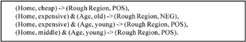
Identification of Minimal RulesDuring the course of rough set-related research, considerable effort was put into development of algorithms for computing minimal rules from decision tables. From a data mining perspective, the rules reflect persistent data patterns representing potentially interesting relations existing between data items. Initially, the focus of the rule acquisition algorithms was on identification of deterministic rules, that is, rules with unique conclusion, and possibilistic rules, that is, rules with an alternative of possible conclusions. More recently, computation of uncertain rules with associated probabilistic certainty factors became of interest, mostly inspired by practical problems existing in the area of data mining where deterministic data relations are rare. In particular, VPRSM is directly applicable to computation of uncertain rules with probabilistic confidence factors. The computation of uncertain rules in VPRSM is essentially using standard rough-set methodology and algorithms involving computation of global coverings, local coverings, or decision matrices (Ziarko & Shan, 1996). The major difference is in the earlier steps of bringing the set of data to the probabilistic decision table form, as described earlier in this chapter. The probabilistic decision table provides an input to the rule computation algorithm. It also provides necessary probabilistic information to associate conditional probability estimates and rule probability estimates with the computed rules. For example, based on the probabilistic decision table given in Table 4, one can identify the deterministic rules by using standard rough-set techniques (see Figure 1).
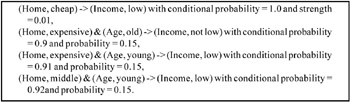
Based on the probabilistic information contained in Table 4, one can associate probabilities and conditional probabilities with the rules. Also, the rough region designations can be translated to reflect the real meaning of the decision, in this case Income = low. The resulting uncertain rules are presented in Figure 2.
All of the above rules have their conditional probabilities within the acceptability limits, as expressed by the parameters l = 0.1 and u = 0.8. The rules for the boundary area are not shown here since they do not meet the acceptability criteria. Some algorithms for rule acquisition within the framework of VPRSM have been implemented in the commercial system DataLogic and in the system KDD-R (Ziarko, 1998b). A comprehensive new system incorporating the newest developments in the rough set area is currently being implemented.
| |||||||||||||||||||||||||||||||||||||||||||||||||||||||||||||||||||||||||||||||||||||||||||||||||||||||||||||||||||||||||||||||||||||||||||||||||||||||||||||||||||||||||||||||||||||||||||
| | |||||||||||||||||||||||||||||||||||||||||||||||||||||||||||||||||||||||||||||||||||||||||||||||||||||||||||||||||||||||||||||||||||||||||||||||||||||||||||||||||||||||||||||||||||||||||||

EAN: 2147483647
Pages: 194