VBA Charting Tricks
This section contains a few charting tricks that I've discovered over the years . Some of these techniques might be useful in your applications, and others are simply for fun. At the very least, studying them could give you some new insights into the object model for charts .
Printing embedded charts on a full page
When an embedded chart is selected, you can print the chart by choosing Office ![]() Print. The embedded chart will be printed on a full page by itself (just as if it were on a chart sheet), yet it will remain an embedded chart.
Print. The embedded chart will be printed on a full page by itself (just as if it were on a chart sheet), yet it will remain an embedded chart.
The following macro prints all embedded charts on the active sheet, and each chart is printed on a full page:
Sub PrintEmbeddedCharts() Dim ChtObj As ChartObject For Each ChtObj In ActiveSheet.ChartObjects ChtObj.Chart.Print Next ChtObj End Sub
Displaying a slide show
The procedure listed below serves as a quick-and-dirty slide show. It displays each embedded chart on the active worksheet in Excel's Print Preview mode. Press Esc or Enter to view the next chart.
Sub ChartSlideShow() Dim ChtObj As ChartObject Application.DisplayFullScreen = True For Each ChtObj In ActiveSheet.ChartObjects Application.ScreenUpdating = False ChtObj.Chart.PrintPreview Next ChtObj Application.DisplayFullScreen = False End Sub
The version below is similar, but it displays all chart sheets in the active workbook.
Sub ChartSlideShow2() Dim Cht As Chart Application.DisplayFullScreen = True For Each Cht In ActiveWorkbook.Charts Application.ScreenUpdating = False Cht.PrintPreview Next Cht Application.DisplayFullScreen = False End Sub
| CD-ROM | The companion CD-ROM contains a workbook that demonstrates a chart slide show. The file is named |
Hiding series by hiding columns
By default, Excel charts don't display data contained in hidden rows or columns. The workbook shown in Figure 18-17 demonstrates an easy way to allow the user to hide and unhide particular chart series. The chart has seven data series, and it's a confusing mess. A few simple macros allow the user to use the ActiveX CheckBox to indicate which series they'd like to view. Figure 18-18 shows the chart with only three series displayed.
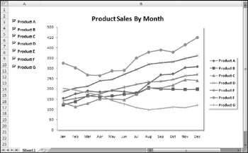
Figure 18-17: Using CheckBox controls to specify which data series to display.
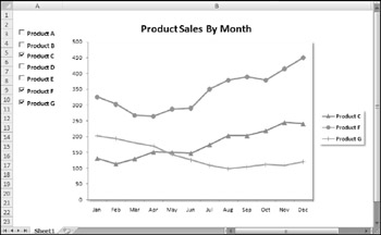
Figure 18-18: A confusing line chart is less confusing when some of the data columns are hidden.
Each series is in a named range: Product_A , Product_B , and so on. Each check box has its own Click event procedure. For example, the procedure that's executed when the user clicks the Product A check box is:
Private Sub CheckBox1_Click() ActiveSheet.Range("Product_A").EntireColumn.Hidden = _ Not ActiveSheet.OLEObjects(1).Object.Value End Sub | CD-ROM | This workbook, named |
Creating unlinked charts
Normally, an Excel chart uses data stored in a range. Change the data in the range, and the chart is updated automatically. In some cases, you might want to unlink the chart from its data ranges and produce a dead chart (a chart that never changes). For example, if you plot data generated by various what-if scenarios, you might want to save a chart that represents some baseline so that you can compare it with other scenarios.
The three ways to create such a chart are:
-
Copy the chart as a picture. Activate the chart and choose Home
 Clipboard
  Paste
Paste  As Picture
  Copy Picture (accept the defaults in the Copy Picture dialog box). Then click a cell and choose Home
  Clipboard
  Paste. The result will be a picture of the copied chart.
 -
Convert the range references to arrays. Click a chart series and then click the formula bar. Press F9 to convert the ranges to an array. Repeat this for each series in the chart.
-
Use VBA to assign an array rather than a range to the XValues or Values properties of the Series object.
The procedure below creates a chart (see Figure 18-19) by using arrays. The data is not stored in the worksheet. As you can see, the SERIES formula contains arrays and not range references.
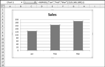
Figure 18-19: This chart uses data from arrays (not stored in a worksheet).
Sub CreateUnlinkedChart() Dim MyChart As Chart Set MyChart = ActiveSheet.Shapes.AddChart.Chart With MyChart .SeriesCollection.NewSeries .SeriesCollection(1).Name = "Sales" .SeriesCollection(1).XValues = Array("Jan", "Feb", "Mar") .SeriesCollection(1).Values = Array(125, 165, 189) .ChartType = xlColumnClustered .SetElement msoElementLegendNone End With End Sub Because Excel imposes a limit to the length of a chart's SERIES formula, this technique works only for relatively small data sets.
The procedure below creates a picture of the active chart (the original chart is not deleted). It works only with embedded charts.
Sub ConvertChartToPicture() Dim Cht As Chart If ActiveChart Is Nothing Then Exit Sub If TypeName(ActiveSheet) = "Chart" Then Exit Sub Set Cht = ActiveChart Cht.CopyPicture Appearance:=xlPrinter, _ Size:=xlScreen, Format:=xlPicture ActiveWindow.RangeSelection.Select ActiveSheet.Paste End Sub
When a chart is converted to a picture, you can create some interesting displays by using the Picture Tools ![]() Format
Format ![]() Picture Styles commands (see Figure 18-20 for an example).
Picture Styles commands (see Figure 18-20 for an example).
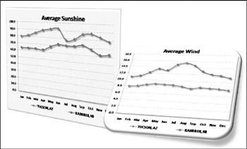
Figure 18-20: After converting a chart to a picture, you can manipulate it by using a variety of commands.
| CD-ROM | The two examples in this section are available on the companion CD-ROM. The filename is unlinked charts.xlsm . |
Displaying text with the MouseOver event
A common charting question deals with modifying chart tips. A chart tip is the small message that appears next to the mouse pointer when you move the mouse over an activated chart. The chart tip displays the chart element name and (for series) the value of the data point. The Chart object model does not expose these chart tips, so there is no way to modify them.
| Tip | To turn chart tips on or off, choose Office |
This section describes an alternative to chart tips. Figure 18-21 shows a column chart that uses the MouseOver event. When the mouse pointer is positioned over a column, the text box (a Shape object) in the upper-left displays information about the data point. The information is stored in a range and can consist of anything you like.
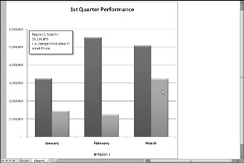
Figure 18-21: A text box displays information about the data point under the mouse pointer.
The event procedure that follows is located in the code module for the Chart sheet that contains the chart.
Private Sub Chart_MouseMove(ByVal Button As Long, ByVal Shift As Long, _ ByVal As Long, ByVal Y As Long) Dim ElementId As Long Dim arg1 As Long, arg2 As Long Dim NewText As String On Error Resume Next ActiveChart.GetChartElement X, Y, ElementId, arg1, arg2 If ElementId = xlSeries Then NewText = Sheets("Sheet1").Range("Comments").Offset(arg2, arg1) Else NewText = "" End If ActiveChart.Shapes(1).TextFrame.Characters.Text = NewText End Sub This procedure monitors all mouse movements on the Chart sheet. The mouse coordinates are contained in the X and Y variables , which are passed to the procedure. The Button and Shift arguments are not used in this procedure.
As in the previous example, the key component in this procedure is the GetChartElement method. If ElementId is xlSeries , the mouse pointer is over a series. The NewText variable then is assigned the text in a particular cell. This text contains descriptive information about the data point (see Figure 18-22). If the mouse pointer is not over a series, the text box is empty. Otherwise, it displays the contents of NewText .
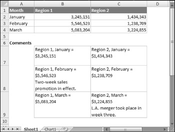
Figure 18-22: Range B7:C9 contains data point information that's displayed in the text box on the chart.
The example workbook also contains a Workbook_Open procedure that turns off the normal ChartTip display, and a Workbook_BeforeClose procedure that turns the settings back on. The Workbook_Open procedure is:
Private Sub Workbook_Open() Application.ShowChartTipNames = False Application.ShowChartTipValues = False End Sub
| CD-ROM | The companion CD-ROM contains this example set up for an embedded chart ( |
EAN: 2147483647
Pages: 319