The Basic Excel Financial Functions
Excel has five basic financial functions: PV, FV, PMT, RATE, and NPER. I discuss each of these functions in this section, and also provide examples.
| Note | All these functions are related in that they are all looking at different sides of the same situation. Many of the arguments are the same from function to function. |
Calculating Present Value
The PV function returns the present value of future cash flows. We know that money in the future has a different value than money today. This function tells us how much that future money is worth right now. Its syntax, with required arguments in bold, is
PV(rate, nper, pmt, fv, type)
The example in this section computes the present value of a series of future receipts, sometimes called an annuity. You get one payment of $1,200 each year for ten years. The value of those payments right now is $6,780.27.
=PV(.12,10,1200,0,0)
In other words, if the payer offered you more than $6,800 right now (so he wouldn't have to make the payments to you in the future), you would take it. If he offered you less, you would pass and wait for the regular payments.
| On the CD | The file |
You may have noticed that in the preceding formula, the interest rate (12%) appeared out of thin air. The PV function is usually used to determine how much a specific future amount is worth today. A specific interest rate is not available in those situations.
| Note | There are a lot of opinions on what discount rate you should use, and which one you choose depends a lot on your personality. Some say that you should use the interest rate you would get from a bank if you borrowed the money with no collateral. Others say you should use the interest rate you would receive if you made a risk-free investment, like in a U.S. Treasury bill. In this example, I use the rate of return you would make if you invested the money in the stock market-because I know you're a shrewd investor. |
The five basic Excel financial functions have many common arguments. The arguments and their meanings are listed here:
-
Rate: The interest rate, expressed as a percentage, that is paid on a loan or used to discount future cash flows.
The period that the interest rate covers must be the same period used for Nper and Pmt.
-
Nper: The number of periods. This could be the number of payments on a loan or the number of years that money is kept in a savings account.
The number of periods must be expressed in the same terms as Rate and Pmt. A 30-year mortgage with monthly payments, for instance, would have an Nper of 360. Three-hundred-sixty months is the number of periods, not 30 years.
-
Pmt: The amount of each payment. For these financial functions, the payments must be the same amount and made at regular intervals.
The payment amount is normally made up of both principal and interest.
-
Fv: The future value. This is the last cash flow that settles the transaction. In many cases, the payments settle the transaction (for example, pay off the loan), so there is no future value.
-
Pv: The present value. This is the first cash flow that starts the transaction, such as borrowing money on a loan or putting money into a savings account.
If the transaction is made up of just payments, there may not be a present value.
-
Type: Whether the payments are made in arrears (0 or default) or in advance (1).
See the preceding section, "Financial Concepts," for more detailed information on Type.
-
Guess: An approximation of the result. When computing an interest rate, Excel must perform many iterations to get the answer.
You can help Excel by specifying a Guess argument that's close to the expected result.
By choosing 12% in this example, I'm saying that you can take the $6,800, invest it so that you make a 12% return, and you'll be in the same financial position as if you had just waited for the $1,200 payments. If the payer offers you $7,000, you can invest that and be in a better position.
Now let's turn the tables and say that you have an obligation to pay someone $1,200 per year for ten years. That formula looks like this:
=PV(.12,10,-1200,0,0)
Instead of a positive cash flow, this formula shows a negative cash flow. The result, $6,780.27, is also oppositely signed from the previous result. In both examples, the sum total of the payments constitutes the entire transaction, so there is no future value. Also, the default value of zero for the Type argument is included. Both the Fv argument and the Type argument are optional, but they are included here for clarity. Figure 11-1 shows these examples in a workbook.
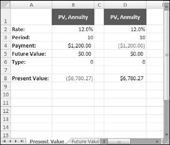
Figure 11-1: Some present value calculations.
| Note | For simplicity, the formulas presented in this chapter use literal values for function arguments. In most cases, you'll use cell references for the arguments. |
| Caution | When entering numeric data as function arguments, make sure that you don't insert thousands separators. For example, type 1000, not 1,000. Depending on your regional settings, the thousands separator may be the same character as the argument separator. |
PRESENT VALUE OF A LUMP SUM
The previous examples dealt with a series of future cash flows, but sometimes there's just one big future cash flow.
For the next example, assume a wealthy relative wants to give you $100,000, but that you can't collect it until your fortieth birthday. If you are 25 years old now, the value of that future gift would be $31,524.17 and is computed as follows:
=PV(.08,15,0,100000)
The payment is an inflow (a positive $100,000) that will occur 15 years from now. If you had some money now, you think you could make 8% investing it. Because there are no payments, the Type argument is irrelevant.
The result of this formula means that if you did have $31,500 now and you invested it at 8%, it would be worth $100,000 in 15 years. See Figure 11-2.
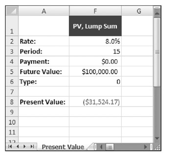
Figure 11-2: Calculating the present value of a lump sum.
PRESENT VALUE OF AN ANNUITY WITH A LUMP SUM
In some cases, future cash flows are followed by a single big future cash flow.
Assume that your brother-in-law wants you to invest in his carpet cleaning business. If you'll invest $50,000 now, he will pay you $200 per month for five years and then also pay you $60,000 at the end of the five years. To determine whether this is a good deal, find the present value of all your future cash inflows:
=PV(.1/12,60,200,60000,1)
Let's look at each of these arguments (see Figure 11-3):
-
You determined that you could make 10% on your money elsewhere, so 10% is the discount rate.
-
All the arguments must cover the same time period. Because the $200 payment is made monthly, all the arguments must be converted to months:
-
The Rate argument is divided by 12 (for 12 months).
-
The Nper argument is expressed as 60 (for 60 months; not 5 for 5 years).
-
-
The payment amount and the lump sum amount were laid out in the deal.
-
The Type argument is 1 because I assume he'll want the first payment now (in advance).
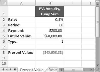
Figure 11-3: Calculating a present value of an annuity with a lump sum.
The formula tells us that the value of all those future cash flows is $45,958.83. According to the terms of this deal and your assumptions, you could make more money investing your $50,000 elsewhere.
| Tip | You can plug in different values for the arguments until you find a solution that is favorable-and then make a counter proposal to your brother-in-law. You can even use Excel's goal seek feature (Data |
Calculating Future Value
The future value is the other side of time value of money coin. It calculates how much a known quantity of money (or a known series of payments) will be worth at some point in the future. The syntax for the FV function follows. Arguments in bold are required arguments.
FV(rate, nper, pmt, pv, type)
FUTURE VALUE OF PAYMENTS
For this example, assume you start a savings account for your new baby's college education. Starting next month, you'll put $50 per month in the account, and you'll earn 3% interest. The formula that follows shows that, in 18 years, the account will have $14,297.02 (see Figure 11-4).
=FV(.03/12,18*12,-50,0,0)
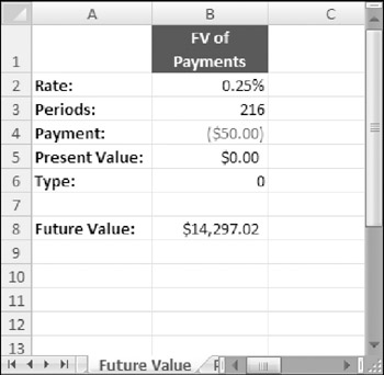
Figure 11-4: Calculating the future value of payments.
The 3% annual percentage rate is converted into a monthly rate, and the 18 years is converted into months. There is no present value because you just opened the account, and the Type is 0 (zero) because you're starting next month (in arrears).
FUTURE VALUE OF A LUMP SUM
The next example computes the future value of a sum of money to which you don't intend to add any money or take any money out.
Assume you roll your 401(k) account into an IRA, but you don't plan to make any more contributions. This formula computes how much your $20,000 will be worth in 15 years when you plan to retire (see Figure 11-5):
=FV(.08,15,0,-20000,0)
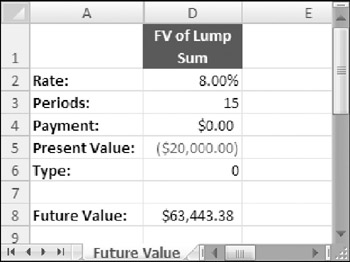
Figure 11-5: Calculating the future value a lump sum.
When you're working with financial formulas, the issue of rounding is almost certain to arise. Excel offers several relevant functions, including ROUND, ROUNDUP, and ROUNDDOWN.
To help prevent cumulative errors, round only the final calculated value. In other words, avoid rounding any intermediate, non-reported calculations.
In general, financial calculations rarely display more than two decimal places, and they often display only full dollar values. For intermediate calculations, this means that you format to the nearest cent (or dollar) and thus retain the fully accurate figure for subsequent calculations.
In some cases, calculations will be based on approximated data or from data based upon subjective opinions or adjusted data (such as rental values), A common professional practice is to report rounded figures to avoid misleading readers. For example, you may have a rental value of $43.55 per square foot, based on an average of recent transactions. If this rate is applied to an area of 1,537 square feet, the calculated rental value is $66,936.35. However, the rental rate is actually an approximation (it may actually be between $42 and $45). To avoid giving an impression of extreme accuracy, you may want to round the calculated rental value to the nearest $100 or even nearest $1,000.
One problem of the accuracy allowed by modern technology is a danger of being seduced by the precision of point estimates.
This example assumes you will average an 8% annual return on your IRA. The –$20,000 represents $20,000 that's flowing away from you and into the IRA. The result, $63,443,38, represents money that's flowing to you from the IRA.
FUTURE VALUE OF PAYMENTS AND A LUMP SUM
It's also possible to compute the future value when there's an existing amount and you plan to add to or subtract from that amount.
In this example, you are going to make monthly payments of $900 against your $150,000 mortgage. If your mortgage interest rate is 5.75%, this formula will compute how much you will still owe on your house in 5 years (see Figure 11-6):
=FV(.0575/12,5*12,-900,150000,0)
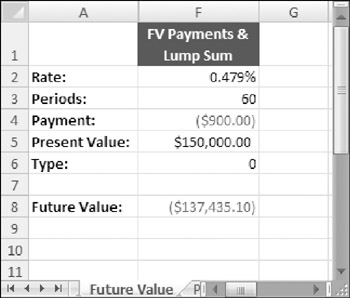
Figure 11-6: Calculating the future value of payments and a lump sum.
The payments are monthly, so the other arguments are converted to months–the annual interest rate is divided by 12, and the Nper expressed in years is multiplied by 12. The current balance of the mortgage is shown as a cash inflow in this example even though no cash is actually flowing in. There was a cash inflow when you originally bought the house.
That is, someone paid you a large sum of money in exchange for a promise to pay it back, and you turned around and bought a house with the money. Because the scope of your problem is from now until five years from now, it doesn't contemplate the time when the funds actually flowed in.
| Tip | One way to think of it is that someone loaned you $150,000 right now to pay off your mortgage, even though that didn't really happen. The –$137,435.10 is the computed outflow to pay that money back at the end of the five years. |
Calculating Payments
The PMT function computes payments required to get a certain balance (pv) down to zero, or some other number (fv). Its syntax is
PMT(rate, nper, pv, fv, type)
COMPUTING LOAN PAYMENTS
When borrowing money, the key question is the periodic payment amount.
In this example, you want to buy a $32,000 car, and you need to compute how much your monthly payments will be. You will make a down payment of $4,000, and the car dealership is offering 2.1% financing for a four-year loan (see Figure 11-7).
=PMT(.021/12,4*12,28000,0,0)
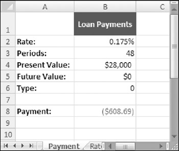
Figure 11-7: Calculating a loan payment.
The formula returns $608.69. So, if you can handle such a monthly outflow, you can get the $28,000 that you borrowed down to zero in 48 payments.
| Caution | If you get a #NUM! error or a result that is obviously incorrect on any of these basic financial functions, the first place to look is the direction of the cash flows. Pay close attention to the signs on the amounts in this section's examples to get a better understanding of how to sign the arguments. |
COMPUTING RETIREMENT PAYMENTS
For some payment calculations, you may have to include a future value amount.
For this example, assume you have $700,000 in a retirement account. If you need to draw out payments to live on for the next 20 years-and still want $100,000 left to leave to heirs-this formula computes how much you can take out every month (see Figure 11-8):
=PMT(.06/12,20*12,-700000,100000,0)
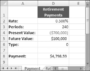
Figure 11-8: Calculating retirement payments.
If your estimated 6% annual return on your money is accurate, you can withdraw $4,798.59 per month, and still have $100,000 in the account 20 years from now.
Calculating Rates
The RATE function computes the interest or discount rate on future cash flows. For transactions where the interest rate is not specifically stated, the RATE function can be used to compute the implicit interest rate (the rate that occurred whether stated or not). Its syntax is
RATE(nper, pmt, pv, fv, type, guess)
PAYDAY LOAN RATES
Payday loans are extremely short-term loans. Generally they are paid back in 14 days (the next paycheck date), and lenders typically charge $15 for every $100 borrowed.
If you borrow $200 and agree to pay $230 in 14 days, the interest rate is calculated with the following formula (see Figure 11-9):
=RATE(1,0,200,-230,0,.01)*365/14
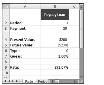
Figure 11-9: Calculating the interest rate on a short-term loan.
The period is set to one because the loan has only one payment. The period of one actually represents a 14-day period, so the rate is converted to an annual percentage rate by dividing by 14 days and multiplying by 365 days. The result, 391%, is so large because the term is so short.
| Note | Interest rates are often stated as annual percentage rates (APRs), even if the term of the loan is more or less than a year. Converting rates to APR, regardless of term, allows you to compare different loans. If you try to compare a monthly interest rate to an annual interest rate, the monthly interest rate will look much smaller but may not actually be. |
GROWTH RATES
A common use of the RATE function is to calculate the growth rate on a retirement account.
Assume for this example that you have a $40,000 balance in your 401(k) at the beginning of the year and $62,000 at the end of the year. You put $200 per paycheck into the account all year (26 payments). This formula shows how your investments performed (see Figure 11-10):
=RATE(26,-200,-40000,62000,0,.01)*26
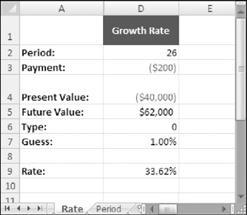
Figure 11-10: Calculating a growth rate.
The RATE function returns the growth rate over each of the 26 periods, so you must multiply it by 26 to get the annual growth rate of 33.62%.
| Note | The Guess argument is used by several financial functions. You can omit this argument and let Excel use the default value, or you can explicitly provide a value. If the result is not close to what it should be, you can try using a different value for the guess argument. |
INTEREST-FREE LOANS
Interest-free loans are rarely free because the interest the merchant would receive for lending you the money is built into the price.
Assume that you want to purchase a $3,000 leather couch, and you can pay for it in 12 monthly payments with no interest. A little comparison shopping reveals that you can get the same couch for $2,500 if you pay cash. So, in essence, you're paying $500 in interest on a $2,500 loan, or 35.07%.
=RATE(12,-3000/12,2500,0,0,.01)*12
You can check the results of the rate function by creating an amortization schedule (see Figure 11-11). If the balance goes to zero, the rate is correct.
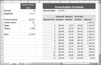
Figure 11-11: An amortization schedule to verify the results of the RATE function.
Calculating Periods
The NPER function is used to determine how many payments are necessary to pay off a loan, or to fund an account to a certain amount. Its syntax is
NPER(rate, pmt, pv, fv, type)
YEARS UNTIL RETIREMENT
If you know how much money you need to retire and you're making regular payments to a retirement account, you can use the NPER function to determine the age at which you can retire.
Assume you'll need $500,000 to retire, and you're putting away $100 per month. Further assume that your retirement account has a balance of $350,000. This formula will return the number of years until you can retire:
=NPER(.1/12,-100,-350000,500000,0)
Assuming you can earn 10% on your investments, NPER returns 41.8 months (or 3.5 years). You can combine NPER and PV if you know how much you need to live on each week, as in this formula:
=NPER(.1/12,-100,-350000,PV(.1/52,20*52,-1000,0,0),0)
The PV function used in the Fv arguments assumes that you'll make 10% (converted to weeks), that you'll need to withdraw money for 20 years (converted to weeks), that you'll need $1,000 per week, and that there will be nothing left. If you can live on $1,000 per week, you can retire in 2.4 years.
The two formulas in this section are shown in Figure 11-12.
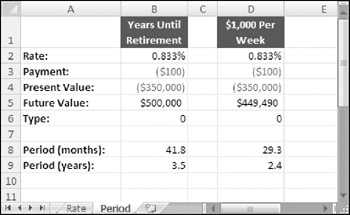
Figure 11-12: Using the NPER function for retirement calculations.
EARLY LOAN PAYOFF
In recent years, many people have refinanced their home mortgages to take advantage of falling interest rates. You can use NPER to calculate how many fewer payments you would have to make due to refinancing.
This example assumes a $200,000 mortgage at 7.5%, with monthly payments of $1,611.19 for the next 20 years. If you refinance to 5.75% but keep making the same payment, this formula computes how many years you can shave off of the loan (see Figure 11-13):
=(20*12)-NPER(.0575/12,PMT(0.075/12,20*12,200000,0),200000,0,0)
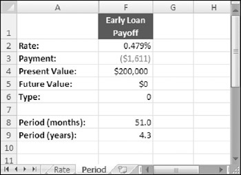
Figure 11-13: Calculating the effect of an early loan payoff.
The pmt argument is a PMT function that computes the $1,611.19 that you're paying based on the terms of your existing mortgage. Subtracting the result from 240 (20 years of 12 months) shows that you can reduce your mortgage term by 51 months by refinancing under these terms.
| Note | Although NPER can produce fraction results (for example, 4.26 months), you probably would not make a payment 26% of the way through a month. Instead, you would make a payment on the fifth month for an amount that's less than the payments you made previously. |
EAN: 2147483647
Pages: 212