21.

[Cover] [Contents] [Index]

Page 116

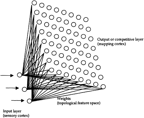
Figure 3.6 Example of the topology of a self-organising map (SOM) with three components: the input layer (sensory cortex) with three neurones, the linking weights (topological feature space), and the output layer (mapping cortex) made up by a grid of 8×8 neurones all equally spaced.

neurone is determined from: min output layer. A competitive Hebbian-type learning law adjusts the synaptic weights of neurone j and its neighbouring neurones:

(3.12)

where the learning rate αⁿ is a time-decaying function (i.e. reducing in magnitude as the number of training iterations increases) expressed as:

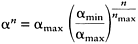(3.13)

with constraints 1≥α, and α_min, α_max≥0. The neighbourhood function βj(γⁿ) determines a Gaussian neighbourhood range centred on the winning neurone j. β_j′ (γⁿ) is calculated by:

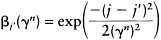(3.14)

[Cover] [Contents] [Index]