206.

[Cover] [Contents] [Index]

Page 283

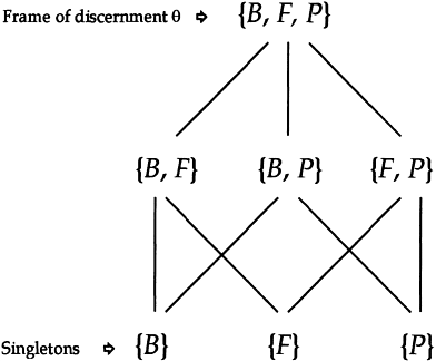
Figure 7.3 A representation of subsets of frame of discernment {B, F, P} made up by bare soil, forest and pasture.

(7.15)

Suppose now one is somewhat uncertain about the reliability of this data evidence and is only willing to commit oneself to label the pixel with, for example, 80% confidence. Then one should change the previous bpa by multiplying each element by 0.8, which leads to:

(7.16)

Note that the quantity of bpa expressed by 6 is denoted by m(θ) and is expressed in this case by:

(7.17)

which is the measure of uncertainty or ignorance; in our case 80% confidence leads to 20% uncertainty and this is reflected in the labelling process.

7.4.2 Belief function and belief interval

In what follows, both the belief function (or support) and the plausibility of each labelling proposition within evidential reasoning are described. A belief function, denoted by Bel, for a hypothesis ψ is defined as the sum

[Cover] [Contents] [Index]