| | 1. | You will build a VI that generates a sine wave array and plots it in a waveform graph. You will also modify the VI to graph multiple plots (see Figure 8.19).
Figure 8.19. Front panel of the VI you will create during this activity 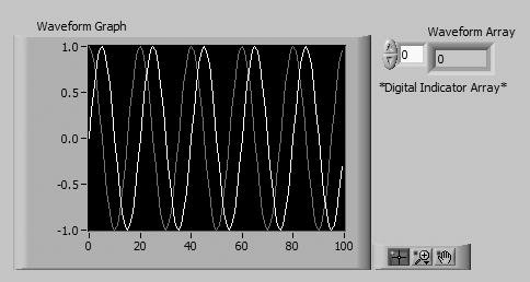
| 2. | Place an array shell (Modern>>Array, Matrix & Cluster palette) in the front panel window. Label the array shell Waveform Array. Place a digital indicator (Numeric palette) inside the Data Object window of the array shell to display the array contents.
| 3. | Place a waveform graph (Modern>>Graph palette) in the front panel window. Label the graph Waveform Graph and enlarge it by dragging a corner with the Positioning tool.
Hide the legend by popping up on the graph and selecting Visible Items>>Plot Legend.
Disable autoscaling by popping up and choosing Y Scale>>AutoScale Y. Modify the Y axis limits by selecting the scale limits with the Labeling tool and entering new numbers; change the Y axis minimum to -1.0 and the maximum to 1.0. We'll talk more about autoscaling in the next section.
| | | 4. | Build the block diagram shown in Figure 8.20.
Figure 8.20. Block diagram of the VI you will create during this activity 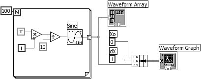
|

Sine Function Sine function (Mathematics>>Elementary & Special Functions>>Trigonometric Functions palette) computes sin(x) and returns one point of a sine wave. The VI requires a scalar index input that it expects in radians. In this exercise, the x input changes with each loop iteration and the plotted result is a sine wave. 
Pi Constant Pi constant (Programming>>Numeric>>Math & Scientific Constants palette). 
Bundle Function Bundle function (Programming>>Cluster & Variant palette) assembles the plot components into a single cluster. The components include the initial X value (0), the delta X value (1), and the Y array (waveform data). Use the Positioning tool to resize the function by dragging either of the resizing handles that appear on the top and bottom edges of the Bundle function as you hover the Positioning tool over it. Each iteration of the For Loop generates one point in a waveform and stores it in the waveform array created at the loop border. After the loop finishes execution, the Bundle function bundles the initial value of X, the delta value for X, and the array for plotting on the graph.
5. | Return to the front panel and run the VI. Right now the graph should show only one plot.
| 6. | Now change the delta X value to 0.5 and the initial X value to 20 and run the VI again. Notice that the graph now displays the same 100 points of data with a starting value of 20 and a delta X of 0.5 for each point (shown on the X axis).
| | | 7. | Place the Positioning tool on the lower-right corner of the array until the tool becomes a grid, and drag. The indicator now displays several elements with indices ascending as you go from left to right (or top to bottom), beginning with the element that corresponds to the specified index, as illustrated in Figure 8.21. (The list of indices below the indicator is a free label used for illustration purposes and won't appear on your panel.) Don't forget that you can view any element in the array simply by entering the index of that element in the index display. If you enter a number greater than the array size, the display will dim.
Figure 8.21. Waveform Array on your VI front panel after running it 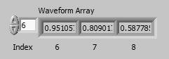
In the block diagram of Figure 8.20, you specified an initial X and a delta X value for the waveform. Frequently, the initial X value will be zero and the delta X value will be 1. In these instances, you can wire the waveform array directly to the waveform graph terminal, as shown in Figure 8.22, and take advantage of the default delta X and initial X values for a graph.
Figure 8.22. Block diagram of your VI after completing step 8 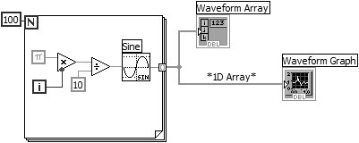
| | | 8. | Return to the block diagram window. Delete the Bundle function and the Numeric Constants wired to it; then select Remove Broken Wires from the Edit menu or use the keyboard shortcut (<control-B> in Windows, <command-B> in Mac OS X, and <meta-B> in Linux). Finish wiring the block diagram as shown in Figure 8.22.
| 9. | Run the VI. Notice that the VI plots the waveform with an initial X value of 0 and a delta X value of 1, just as it did before, with a lot less effort on your part to build the VI.
|
Multiple-Plot Graphs You can also create multiple-plot waveform graphs by wiring the data types normally passed to a single-plot graph, first to a Build Array function, and then to the graph. Although you can't build an array of arrays, you can create a 2D array with each input array as a row. 10. | Create the block diagram shown in Figure 8.23.
|
Figure 8.23. Your VI after adding an additional plot 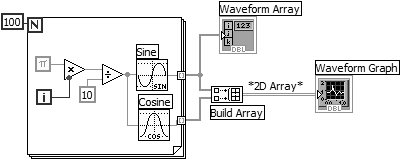

Build Array Function Build Array function (Programming>>Array palette) creates the proper data structure to plot two arrays on a waveform graph. Enlarge the Build Array function to include two inputs by dragging a corner with the Positioning tool. You will want to make sure you don't select "concatenate inputs" (just use the default value selected in the pop-up menu) to the Build Array so the output will be a 2D array. If you wish to do so, you can review the "concatenate inputs" feature of the Build Array node in Chapter 7. 
Cosine Function Cosine function (Mathematics>>Elementary & Special Functions>>Trigonometric Functions palette) computes cos (x) and returns one point of a cosine wave. The VI requires a scalar index input that it expects in radians. In this exercise, the x input changes with each loop iteration and the plotted result is a cosine wave. | | 11. | Switch to the front panel. Run the VI. Notice that the two waveforms both plot on the same waveform graph. The initial X value defaults to 0 and the delta X value defaults to 1 for both data sets.
| 12. | Just to see what happens, pop up on the graph and choose Transpose Array. The plot changes drastically when you swap the rows with the columns, doesn't it? Choose Transpose Array again to return things to normal.
| 13. | Save and close the VI. Name it Graph Sine Array.vi in your MYWORK directory or VI library.
|
|