THE DATA WAREHOUSE ARCHITECTURE
| only for RuBoard - do not distribute or recompile |
THE DATA WAREHOUSE ARCHITECTURE
There has been considerable discussion in the industry about the various approaches to the development of data warehouses.
After some successful projects, and some more spectacular failures, the discussion has tended to focus on the benefits of data marts, or application-centric information systems, sometimes referred to as department-level data warehouses. The rationale around these ideas is that enterprise data warehouses are high-risk ventures that, often, do not justify the expense and extended delivery times. A department-level data mart, on the other hand, can be implemented quickly, easily, and with relatively low risk.
The big drawback of department-level information systems is that they almost always end up as stove -pipe developments. There is no consistency in their approach, and there is usually no way to integrate the data so that anything approaching enterprise-wide questions can be asked. They are attractive because they are low risk. They are low risk because they incur relatively low cost. The benefits they bring are equally quite low.
What we need are information systems that help the business in pursuit of its goals. As the goals evolve, the information systems evolve as well. Now that's a data warehouse! The trick is to adopt a fairly low risk, and low cost, approach with the ultimate result being a complete and fully integrated system. We do this by adopting an incremental approach. The benefits of an incremental approach to delivering information systems are recognized and I am an enthusiastic exponent of this approach, as long as it is consistent with business goals and objectives. In order to do this we need to have a look back at the idea behind database systems.
The popular introduction of database management systems in the 1970s heralded the so-called Copernican revolution in the perception of the value of data. There was a shift in emphasis away from application centric toward a more data centric approach to developing systems. The main objectives of database management systems are the improvement of:
-
Evolvability. The ability of the database to adapt to the changing needs of the organization and the user community. This includes the ability of the database to grow in scale, in terms of data volumes , applications, and users.
-
Availability. Ensuring that the data has structure, and is able to be viewed in different ways by different applications and users with specific and nonspecific requirements.
-
Sharability. Recognition of the fact that the data belongs to the whole organization and not to single users or groups of users.
-
Integrity. Improving the quality, maintaining existence, and ensuring privacy.
The degree to which success has been achieved is a moot point. Some systems are better, in these respects, than others. It would be difficult to argue that some of the online analytical processing (OLAP) systems with proprietary database structures achieve any of the four criteria in enterprise-wide terms.
The point here is that, even with sophisticated database management systems now at our disposal, we are still guilty of developing application-centric systems in which the data cannot easily be accessed by other applications.
Where operational, or transactional, systems are concerned this appears to be acceptable. In these cases the system boundaries seem to be clear, and it could be argued that there is no need for other systems to have access to the data used by the application. Where such interfaces are found to be of benefit, integration processes can be built to enable the interchange of information.
With informational systems, however, the restriction is not acceptable.
It is also not acceptable where transactional systems are required to provide data feeds to informational systems if the transactional data is structured in such a way that it cannot be easily read using the standard query language provided by the DBMS.
These practices do nothing to smooth the development of informational systems and contribute to the risk of embarking on any decision support project.
The objectives of evolvability, availability, sharability, and integrity are still entirely valid and even more so with decision support systems where the following exists:
-
The nature of the user access tends to be unstructured.
-
The information is required for a wide number of users with differing needs.
-
The system must be able to respond to changes in business direction in a timely fashion.
-
The results of queries must be reliable and consistent.
The development of an application-centric solution will not support those objectives. The only way to be sure that the database possesses these qualities is to design them in at the beginning.
This requirement has given rise to the EASI (evolvability and availability, sharability, integrity) data architecture, an example of which is shown in Figure 7.1.
Figure 7.1. The EASI data architecture.
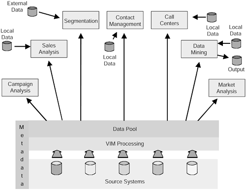
The foundation of EASI is the data pool. The data pool contains the lowest level of detail (granularity) of data that the organization is able to store. Ideally, this should be at transaction level. The data pool is fed by the organization's operational systems.
The data pool supports the information and decision support systems (applications) that are able to take data from the pool, as well as store data of their own.
The applications are entirely independent of one another and have their own users and processing cycles.
The applications can, in turn , provide data to other systems or can even update the source systems.
The most important point to note is that the data pool is a resource that is available to all applications. This is entirely consistent with the original objectives of database management systems.
The various components of the model are now described in more detail.
The VIM Layer
In order for data to be allowed to enter the pool, each item of data must conform to rigorous constraints regarding its structure and integrity. Every data item must pass through a series of processing steps known as VIM (see Figure 7.1). VIM stands for validation, integration, and mapping. Collectively the VIM processes form the basis of the data quality assurance strategy for the data warehouse.
Closely associated with the VIM processing is a comprehensive metadata layer. We will be building the metadata as we go.
Data Validation
The validation layer is the first part of the data quality assurance process. The validation of data is one of the most important steps in the loading of data into the warehouse. Although this might sound obvious, it is one area that is often hopelessly underestimated in the planning of a data warehouse. Unfortunately, when we ask the question, What is the quality of your data? the answer is invariably that their data is nearly 100 percent perfect. This assertion is always wrong. Most organizations have no clue about the quality of their data and are always na ve in this respect. If they say it's near perfect, you can be sure that it's poor. If they admit to their data being OK then it's likely to be desperately poor.
Clearly, if the quality of data is poor, then the accuracy of any information that can be derived from it will be highly suspect. We cannot allow business decisions to be based on information of questionable accuracy. Once it becomes known that the accuracy of the information cannot be relied upon, the users will lose trust in the data warehouse and will stop using it. When this happens, you might as well shut it down.
There are several classes of data quality issues. Data can be:
-
Missing (or partially missing)
-
Erroneous
-
Out of date
-
Inconsistent
-
Misleading
Missing data. The main reason for data to be missing is insufficient rigor in the routine data collection processes of the operational systems. This might be fields on an input screen or document where, for the purposes of the application, the data is not classified as mandatory whereas in the warehouse environment, it is absolutely mandatory. An example of this, insofar as the Wine Club is concerned, might be the customer's favorite hobby. When a new customer is registered, the data entry operator might not appreciate the value of this piece of information and, unless they are forced to, might not capture the information. In our CRM solution, we are trying hard to tailor our products and services toward our customers' preferences, and the absence of information will make it all the harder for us to do this successfully.
Resolving the issue of missing data can be a nightmare. Ideally, the missing values should be sorted out within the source system before the data is extracted and transferred to the warehouse. Sometimes this is not possible to do and sometimes it is not desirable, and so the warehouse design has to incorporate some method of resolving this.
It is very risky to allow data into the warehouse with missing values, especially if it results in null values. Here is an example. Take a look at the fragment of the customer table in Table 7.1.
Table 7.1. Table Containing Null Values
| Customer ID | Customer Name | Salary |
|---|---|---|
| 12LJ49 | Lucie Jones | 20,000 |
| 07EK23 | Emma Kaye | null |
| 34GH54 | Ginnie Harris | 30,000 |
| 45MW22 | Michael Winfield | 10,000 |
| 21HL11 | Hannah Lowe | null |
Now consider the queries shown in Table 7.2.
Table 7.2. Query Results Affected by Null Values
| Query | Result |
|---|---|
| Select count(*) from customer | 5 |
| Select count(Salary) from customer | 3 |
| Select min(Salary) from customer | 10,000 |
| Select avg(Salary) from customer | 20,000 |
Although these results are technically correct, in business terms, apart from the first, they are clearly wrong. While it is reasonable to say that we might be able to spot such errors in a table containing just five rows, how confident are we that such problems could be detected in a table that has several million rows?
The approach to the correction of missing values is a business issue. What importance does the business place on this particular data element? Where there is a high level of value placed on it, then we have to have some defined process for dealing with records where the values are missing. There are two main approaches:
-
Use a default value.
-
Reject the record.
Use of default values means that the rejection of records can be avoided. They can be used quite effectively on enumerated or text fields and in foreign key fields. We can simply use the term unknown as our default. In the case of foreign keys, we then need to add a record in the lookup table with a primary key of UN and a corresponding description. The example of the hobbies table in Table 7.3. makes this clear.
Table 7.3. The Wine Club Hobbies Table
| Hobby Code | Hobby Description |
|---|---|
| GF | Golf |
| HR | Horse riding |
| MR | Motor racing |
| UN | Unknown |
A fragment of the customer table is shown again in Table 7.4.
Table 7.4. Part of the Customer Table
| Customer ID | Customer Name | Hobby Code |
|---|---|---|
| 12LJ49 | Lucie Jones | MR |
| 07EK23 | Emma Kaye | UN |
| 34GH54 | Ginnie Harris | GF |
| 45MW22 | Michael Winfield | GF |
| 21HL11 | Hannah Lowe | UN |
A query to show the distribution of customers by hobby will result in Table 7.5.
Table 7.5. Result of the Query on Customers and Their Hobbies
| Hobby Description | Count(*) |
|---|---|
| Golf | 2 |
| Motor Racing | 1 |
| Unknown | 2 |
A benefit of default values is that we can always see the extent to which the default has been applied. The application of defaults should, however, be limited to sets of a known size .
If we have, say, 50 different hobbies it is easy to imagine adding a further unknown category. In the previous example, salary, how can we possibly define a default value, other than null, to be used when the column has continuous values? We cannot apply a text value of unknown to a numeric field. The only way to deal with this effectively is to prevent such a record from getting into the warehouse. So we reject them.
Rejecting records means that they are not allowed into the warehouse in their current state. There are three main approaches to the rejection of records:
Permanent rejection. In this situation, the record is simply thrown away and never gets into the warehouse. The obvious problem with this solution is that there is a compromise of simplicity of operation versus accuracy of information. Where the volumes are tiny in proportion to the whole, this might be acceptable but extreme care should be exercised. This type of solution can be applied only to behavioral records, such as sales records, telephone calls, etc. It should not be applied to records relating to circumstances. For instance, if we were to reject a customer record permanently because the address was missing, then every subsequent sale to that customer would also have to be rejected because there would be no customer master record to match it up to.
Reject for fixing and resubmission. With this approach, the offending records are sidelined into a separate file that is subjected to some remedial processing. Once the problems have been fixed, the records are reentered into the warehouse. The simplest way to do this is to merge the corrected records with the next batch of records to be collected from the operational system so that they get automatically revalidated as before. This sounds like a neat solution and it is. Beware however. Firstly, if we take this approach, it means that we have to build a set of processes, almost a subsystem, to handle the rejections, allow them to be modified somehow, and place them back in the queue. This system should have some kind of audit control so that any changes made to data can be traced, as there is a clear security implication here. The mechanism we might adopt to correct the records could be a nice windows -style graphical user interface (GUI) system where each record is processed sequentially by one or more operators. Sometimes the rejection is caused by an enhancement or upgrade to the source system that ever so slightly changes the records that are received by the data warehouse. When this happens, two things occur. First, we do not see the odd rejection; we see thousands or millions of rejections. Second, if the format of the records has changed, they are unlikely to fit into the neat screen layouts that we have designed to correct them. The reject file contains some true records and a whole pile of garbage. This situation really requires a restore and a rerun. Restores and reruns are problematic in data warehousing. We will be covering this subject later in the chapter.
Reject with automatic resubmission. This is a kind of variation on the previous type of rejection. Sometimes, simply resubmitting the offending record is sufficient. An example of this occurs frequently in mobile telecommunication applications. The customer Lucie Jones goes into her local telephone store, orders a new service, and 15 minutes later leaves the store with her new possession. Almost immediately the telephone is activated for use and Lucie is able to make calls. That evening, all the calls that Lucie has made will be processed through the mediation system through to billing and will then be transferred to the data warehouse. However, Lucie's circumstances (customer details), name, address, billing information, etc., are unlikely to find their way to the data warehouse in time to match up to her telephone calls. The missing data, in this example, are Lucie's customer details. The result is that Lucie's calls will be rejected by the warehouse as it does not have a customer with whom to match them up. But we don't want them to be passed to some manual remedial process to correct them. What we need is for the calls to be recycled and re-presented to the validation process until such time as Lucie's master customer record turns up in the data warehouse. When this happens, the calls will be accepted without further intervention. Clearly there has to be a limit to the number of cycles so that records that will never become valid can be dealt with in another way.
Each of the three approaches to the rejection of records can be adopted or not, depending on what is best for the business. In some organizations, all three approaches will be used in different parts of the application.
The important point to note is that, although the rejection of records seems like an easy solution to the problem of missing data, a considerable amount of processing has to be built around the subsequent handling of those records.
Erroneous Data. Whereas missing data is easy to spot, data that is present but that is simply wrong can sometimes be harder to detect and deal with. Again, there are several types of erroneous data:
Values out of valid range. These are usually easy to recognize. This type of error occurs when, say, the sex of a customer, which should have a domain of F or M contains a different value, such as X. It can also apply to numerical values such as age. Valid ages might be defined as being between 18 and 100 years . Where an age falls outside of this range, it is deemed to be in error.
Referential errors. This is any error that violates some referential integrity constraint. A record is presented with a foreign key that does not match up to any master record. This is similar to the problem we described in the previous section. This could occur if, say, a customer record were to be deleted and subsequent transaction records have nothing to match up to. This kind of problem should not be encountered if the guidelines on deletions, which were described in Chapter 6, are followed. However, this does not mean that referential integrity errors will not occur; they will. How they are dealt with is a matter of internal policy, but it is strongly recommended that records containing referential errors are not allowed into the warehouse because, once in, they are hard to find and will be a major cause of inconsistency in results.
As an example, look at the slightly modified customer table in Table 7.6.
Table 7.6. Customer Table Fragment Containing Modified Hobby Codes
| Customer ID | Customer Name | Hobby Code |
|---|---|---|
| 12LJ49 | Lucie Jones | MR |
| 07EK23 | Emma Kaye | OP |
| 34GH54 | Ginnie Harris | GF |
| 45MW22 | Michael Winfield | GF |
| 21HL11 | Hannah Lowe | OP |
Now, instead of having hobby codes of UN (unknown), Emma and Hannah have codes relating to opera as their hobby. A simple query to group customers by hobby is as follows :
Select HobbyDescription, Count(*) From Customer C, Hobby H Where C.HobbyCode = H.HobbyCode Group by HobbyDescription
Table 7.7 is the result.
Table 7.7. Result Set With Missing Entries
| Hobby Description | Count(*) |
|---|---|
| Golf | 2 |
| Motor racing | 1 |
Emma and Hannah have disappeared from the results. What may be worse is that all of their behavioral data will also be missing from any query that joined the customer table to a fact table.
The best way to deal with this type of referential integrity error is to reject the records for remedial processing and resubmission.
Valid errors. These are errors in the data that are almost impossible to detect: values that have simply been entered incorrectly, but that are still valid. For instance, a customer's age being recorded as 26 when it should be 62. Typically, errors like this are made in the operational systems that supply the data warehouse and it is in the operational systems that the corrections should be made. In many cases, corrections are ad hoc, relying on sharp-eyed operators or account managers who know their customers and can sometimes, therefore, spot the errors.
We can sometimes take a more proactive approach by, periodically, sending data sheets to our customers that contain their latest details, together with an incentive for them to return the information with any corrections.
Out-of-Date Data. Out-of-date information in a data warehouse is generally the result of too low a frequency of synchronization of customers' changing circumstances between the operational systems and the warehouse. An example is where a customer's change of address has been recorded in the operational system but not yet recorded in the data warehouse. This problem was covered in some detail in Chapter 4. The conclusion was that we should try to receive changes from the operational systems into the warehouse as frequently as possible.
Inconsistent Data. Inconsistent data in the data warehouse is a result of dependencies, or causal changes, of which the operational systems may be ignorant. For instance, we may be maintaining a derived regional segment based on customer addresses. This segmentation is held only within the data warehouse and is not known by the operational system. When a customer moves from one address to another, eventually the data warehouse has to be informed about this and will, routinely, make the appropriate adjustment to the customer's circumstances. The regional segment, and any other address-dependent segments, must also be updated. This is a change that is solely under the control of the data warehouse and its management and systems. This can be quite a headache because the segments are dynamic. New ones appear and old ones disappear. The causal effect of changes to circumstances, on the various segments that are dependent on them, is a hard nut to crack.
Misleading Data. Misleading data can occur when apparent retrospective changes are made and the representation of time is not correct. This was explained in Chapter 4. An example is where a change of address occurs and, due to the incorrect application of retrospection, the new address is erroneously applied to historical behavioral data. Oddly enough, the reverse situation also applies. When describing so-called valid errors, the example was where the customer's age was recorded as 26 but should have been 62. If we had classified the age of the customer as having true retrospection, then any correction might have been implemented such that, at a particular point in time, the customer's age jumped from 26 years to 62 years. In this case, it is the proper use of retrospection that causes the data to be misleading.
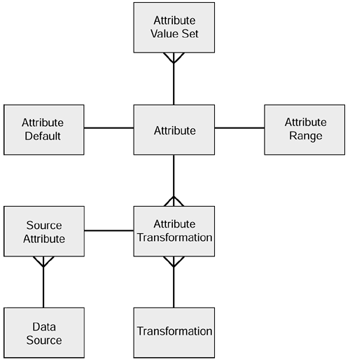
In order to provide a flexible approach to validation, we should build our validation rules, as far as is practical, into our metadata model. An example of a simple validation metadata model for validation is shown in Figure 7.2.
Figure 7.2. Metadata model for validation.
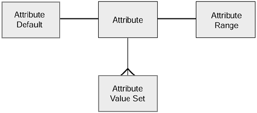
The attributes of the validation metadata tables are as follows:
| Attribute Table | |
|---|---|
| Attribute ID | |
| Table name | |
| Attribute name | |
| Data type | |
| Retrospection | |
| Attribute Default Table | |
| Attribute ID | |
| Default value | |
| Attribute Range Table | |
| Attribute ID | |
| Lowest value | |
| Highest value | |
| Attribute Value Set Table | |
| Attribute ID | |
| Value | |
The data that is held in the default value, lowest value, and highest value columns is fairly obvious. It is worth noting that, in order to make it implementable, all values, including numerics, must be held as character data types in the metadata tables. So the DDL for the default value table would be:
Create table Attribute_Default ( Attribute_ID number (6), Default_Value Varchar(256))
An example of some of the entries might be:
| Attribute Table | |||
|---|---|---|---|
| Attribute ID: | 212 | 476 | |
| Table name | Customer | Customer | |
| Attribute name | Occupation | Salary | |
| Target data type | Char | Num | |
| Retrospection | False | True | |
| Attribute Default Table | |||
| Attribute ID | 212 | 476 | |
| Default value | Unknown | 15,000 | |
This shows that the default value, although numeric, is stored in character format. Obviously in the customer table the salaries will be stored as numerics, and so some format conversion, determined by examination of the target data type attribute, will have to be performed whenever the default value is applied. Lastly, the attribute value set is just a list of valid values that the attribute may adopt.
Integration
The next part of the VIM processing is the integration layer. The integration layer ensures that the format of the data is correct. Format integrity means that, for instance, dates all look the same (e.g., yyyymmdd format), or maybe product codes from some systems might need to be converted to comply with a standard view of products.
For many attributes there may be no problem. Where data formats are standard throughout an organization, there is little need to manipulate and transform the data so long as the standard is itself a form that enables data warehouse types of queries to be performed. In order to make the integration as flexible as possible, as much as possible should be implemented in metadata. So we need to extend our metadata model so that it can be used for integration. The extensions are shown in Figure 7.3.
Figure 7.3. Integration layer.
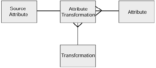
| Attribute Table | |
|---|---|
| Attribute ID | |
| Table name | |
| Attribute name | |
| Data type | |
| Data format | |
| Business description | |
| Source Attribute Table | |
| Source attribute ID | |
| Source attribute name | |
| Data type | |
| Data format | |
| Business description | |
| Transformation Table | |
| Transformation process ID | |
| Transformation process name | |
| Transformation process type | |
| Transformation description | |
| Attribute Transformation Table | |
| Attribute ID | |
| Source attribute ID | |
| Transformation process ID | |
The attributes of the validation metadata tables are as follows:
The attribute table has been extended to accommodate the additional requirements of the integration part of the VIM processing. Of course, there are many more attributes that could be included, but this approach is quite flexible and should be able to accommodate most requirements.
These tables can form an active part of the VIM process. As an example, the attribute table would contain an entry for the sex of the customer. The source system might not contain such an attribute, but we might be able to derive the sex from the customers' title ( Mr. translates to Male while Mrs., Ms, and Miss translate to Female ). The source attribute would be the title of the customer in the customer database. The transformation process held in the transformation table would be the routine that made the translation from title to sex. Then the attribute transformation table brings these three things together. The VIM process can now determine:
-
Source attribute (title from customer data)
-
Process to transform it
-
Target attribute (customer's sex)
The great attraction of this approach is that it is entirely data driven. We can alter any of the three components without affecting the other two.
Mapping
The mapping layer is a data-driven process that takes source data and maps it to the target format. The purpose of this approach is to ease the transition when we are required, for instance, to replace one source system with another or to accept altered data feeds. The aim is to develop a formal mapping layer that makes it easy to implement changes in sources where no additional functionality is being added (e.g., as a result of source system upgrades).
The changes to the metadata model to accommodate this are quite small. We can simply add a source entity to the previous model as shown in Figure 7.4.
Figure 7.4. Additions to the metadata model to include the source mapping layer.
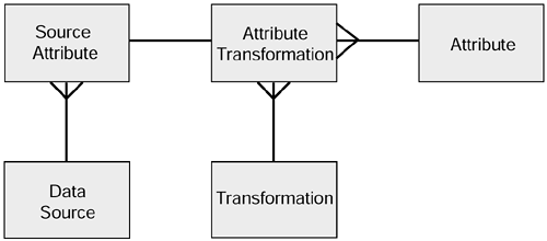
The attributes for the source are as follows:
| Data Source Table | |
|---|---|
| Source ID | |
| Source name | |
| Source application | |
| File type | |
| Interface format | |
| Source platform | |
| Extraction process | |
| Extraction frequency | |
| Business description | |
| Source Attribute Table | |
| Source ID | |
| Source attribute ID | |
| Source attribute name | |
| Data type | |
| Data format | |
| Business description | |
The complete metadata model for the VIM process is shown in Figure 7.5.
Figure 7.5. Metadata model for the VIM layer.
Margin of Error
In Chapter 4, we said our users had no real way of knowing whether their query results were adversely affected by the inadequate representation of time.
In this section we'll look at a margin of error calculation that could be provided as a standard facility for data warehouses. The proposal is that information regarding retrospection and time lags is held in a metadata table so that any query can be assessed as to the likely margin of error.
There are two main components to the margin of error:
-
The degree to which the dimensions are subject to change. In order to be entirely accurate, the problem must be approached on a per attribute basis. Different attributes will change at differing rates, and so it is not sensible to view the likelihood of change at the entity level.
-
The transaction time 1 to transaction time 2 lag. This component covers the error caused by changes that have been recorded in the operational system but not yet been captured into the data warehouse. Transaction time 1 is the time when the data is recorded in the operational system. Transaction time 2 is the time when the change is notified to the data warehouse.
The first of these two can be eliminated if the requirement for retrospection, for the attribute, has been implemented properly. The second can be eliminated only if the valid time to transaction time lag is eliminated.
The period of the query will also affect the accuracy. If 10 percent of customers change their address each year, then the longer the period, the greater the potential for error.
The following formula can be used to calculate the percentage error for an attribute in the data warehouse.

where:
-
T is the time period, in years, covered by the query.
-
C is the percentage change per annum. So, if the attribute is an address, and 10 percent of people change their address each year, then C is 10.
-
R is the value for retrospection. It has a value of 0 (zero) where true retrospection has been implemented, or 1 (one) where true retrospection has not been implemented.
-
L is the average time lag, in days, between transaction time 1 and transaction time 2 .
The total percentage margin of error in a query is calculated by summing the individual attribute percentages. It is important to understand what the error% actually provides. It is the percentage of rows accessed during the query that may be in error. It is not a percentage that should be applied to the monetary or quantitative values returned by the query.
This method is implemented by the creation of a metadata table called Error_Stats that has the following attributes:
-
Table name
-
Column name
-
Time lag
-
Retrospection
-
Change percent
The table is then populated with entries for each attribute, as Table 7.8 shows.
Table 7.8. Example Error_Stats Table
| Table Name | Column Name | Time Lag | Retrospection | Change Percent |
|---|---|---|---|---|
| Customer | Address | 30 | 10 | |
| Customer | Sales_Area | 30 | 10 | |
| Wine | Supplier_Code | 7 | 1 | 20 |
If it is required to estimate the margin of error that should be applied to a query involving Address and Supplier_code columns, the following query could be executed against the Error Stats metadata table:
select sum(change_pct*((1.5*retrospection) +(time_lag/365))) "Error Pct" from error_stats where (table_name='Customer' and column_name='Address') or (table_name='Wine' and column_name='Supplier_Code)
The 1.5 means that the query will embrace a period of one and a half years. The query returns the result in Table 7.9.
Table 7.9. Example Margin of Error
| Error Pct |
|---|
| 31.21 |
Table 7.9 indicates a 31 percent margin of error. Most of this is due to the fact that true retrospection has not been implemented on the supplier code, which, having a 20 percent change factor, is quite a volatile attribute.
It is envisaged that a software application would be developed so that users of the data warehouse would not have to code the SQL statement shown above. All that would be needed is to select an option called, perhaps, Margin of Error after having selected the information they want to retrieve. The software application would extract the columns being selected and determine the time period involved. It would then build the above query and inform the user of the estimated margin of error.
This attempt at calculating the margin of error is, it is believed, the first attempt at enabling users of data warehouses to assess the accuracy of the results they obtain. There is a limit to the degree of accuracy that can be achieved, and it must be recognized that valid times are often impossible to record as they are often not controlled by the organization but are under the control of external parties such as customers and suppliers.
In order to minimize inaccuracy, the period of time between valid time and transaction time 1 , and between transaction time 1 and transaction time 2 , should be as short a time as is possible.
The possible range of results of the formula needs some explaining. When using the formula, a result of much greater than a 100 percent margin of error can be returned. This might sound daft, but actually it's not. Let's reexamine the example, which, having been used before in this book ad nauseum, states that 10 percent of people move house each year. After one year, 10 percent of our customer records are likely to have changed. This means that if we haven't implemented true retrospection, then 10 percent of the rows returned in queries that use the address can be regarded as being of questionable accuracy. After 10 years, the figure rises to 100 percent. But what happens after 11 years, or 15 years, or more? It is fair to say that any result returned by the formula that indicates a margin of error of more than, say, 15 percent should be regarded as risky. Anything beyond 30 percent is just plain gobbledeygook.
Data Pool
The data pool can be regarded as the physical manifestation of the GCM. Obviously, the physical model may be very similar or very dissimilar to the original conceptual model. Many compromises may have to be made depending on the underlying DBMS and the need to balance the business requirements with considerations regarding performance and usability. For the purposes of this book, we will assume that the DBMS will be relational and we will keep the general shape of the GCM as far as possible.
As previously stated, the data pool is independent of any decision support application. It is held at the lowest level of granularity that the organization can support. Ideally, behavioral data should be stored at transaction level rather than having been summarized before storing.
Data can be allowed into the pool only after it has passed through the VIM processing just described.
In order to describe the data pool fully, we will construct it using the Wine Club example. Firstly, let's look at the customers' fixed (retrospection is false or permanent) circumstances, shown in Figure 7.6.
Figure 7.6. Customer nonchanging details.

The attributes associated with this are:
| Customer Table | |
|---|---|
| Title | |
| Name | |
| Date of birth | |
| Sex | |
| Telephone number | |
Next, to the customer data in Figure 7.6 we add the design for the changing (retrospection is true) circumstances. Not surprisingly, this is the same diagram as we produced in Chapter 3 (Figure 3.13). The result is shown in Figure 7.7.
Figure 7.7. The changing circumstances part of the GCM.
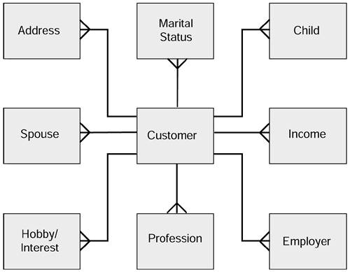
The attributes of the changing circumstances tables are as follows:
| Address Table | |
|---|---|
| Customer ID | |
| Address | |
| Start date | |
| End date | |
| Marital Status Table | |
| Customer ID | |
| Marital status | |
| Start date | |
| End date | |
| Child Table | |
| Customer ID | |
| Child name | |
| Child date of birth | |
| Spouse Table | |
| Customer ID | |
| Spouse name | |
| Spouse date of birth | |
| Income Table | |
| Customer ID | |
| Income | |
| Start date | |
| End date | |
| Hobby Table | |
| Customer ID | |
| Hobby | |
| Start date | |
| End date | |
| Profession Table | |
| Customer ID | |
| Profession | |
| Start date | |
| End date | |
| Employer Table | |
| Customer ID | |
| Employer name | |
| Employer address | |
| Employer business category | |
| Start date | |
| End date | |
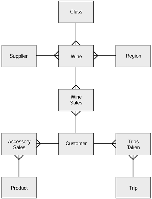
Next, we assemble the behavioral model. In the Wine Club, we just want:
-
Sales of wine
-
Sales of accessories
-
Trips taken
The model for this is as shown in Figure 7.8.
Figure 7.8. Behavioral model for the Wine Club.
Finally, we need to design the last part of the model, the derived segments. The model for this is shown in Figure 7.9.
Figure 7.9. Data model for derived segments.
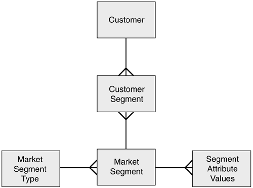
The attributes for these tables, together with examples, are shown in Table 7.10.
Table 7.10. Example of Segmentation
| Market Segment Type Table | ||
|---|---|---|
| Market segment type ID | LT217 | |
| Market segment type description | "Income Segment" | |
| Market Segment Table | ||
| Market segment type ID | LT217 | LT217 |
| Market segment ID | 04 | 05 |
| Market segment description | "Middle Earner" | High Earner |
| Segment Attribute Values Table | ||
| Market segment type ID | LT217 | LT217 |
| Market segment ID | 04 | 05 |
| Table | "Customer Salary" | Customer Salary |
| Attribute | Salary | Salary |
| Attribute low value | 30,001 | 50,001 |
| Attribute high value | 50,000 | 75,000 |
| Customer Segment Table | ||
| Customer ID | 12LJ49 | L2LJ49 |
| Market segment type ID | LT217 | LT217 |
| Market segment ID | 04 | 05 |
| Start date | 21 Jun 1999 | 1 Mar 2001 |
| End date | 28 Feb 2001 | null |
The example shows Lucie Jones's entries in the customer segment table as moving from a middle earner to a high earner. You can see, from Figure 7.9 and the example in Table 7.10, that a market segment can be made up of many segment attribute values. The attribute values can be drawn from any table that contains customer information. Therefore, the customer segment table itself could be referred to in the definition of a market segment. This means that Lucie's improving status, as shown by her moving from 04 to 05, might itself be used in positioning her in other segments, such as Customer Lifetime Value.
So, now we have built all the main components of the Wine Club's data pool. Firstly there is the customer, the single entity shown in Figure 7.6. Then we have the customers' changing circumstances in Figure 7.7. Next, from Figure 7.8 we add the customer behavior and, finally, we have a neat way of recording customers' derived segments, and this is shown in Figure 7.9.
These four components, when fitted together, are the Wine Club's physical representation of the GCM that we have been working with throughout this book.
Of course there is more work to be done. For instance, in the behavioral model we have focused only on the customer. For each of the dimensional models we have created, we would expect to see may more dimensions than we have drawn. Each of the dimensions would be subjected to the same rigourous analysis as the customer information part. Even so, we have achieved a lot.
Consider the problems we have had to tackle. First, the requirement to support customer circumstances as well as behavior so that we can do sensible predictive modeling for things like customer churn. This model does that. Then there were the huge problems brought about by poor representation of time. This model overcomes that too, it can handle all three types of temporal query. The behavioral stuff is still in the form of dimensional models, but overall, the model can truly be described as customer centric.
Now that we have dealt with the data architecture for the pool, we'll briefly mention the applications.
| only for RuBoard - do not distribute or recompile |
EAN: 2147483647
Pages: 96
- Challenging the Unpredictable: Changeable Order Management Systems
- ERP System Acquisition: A Process Model and Results From an Austrian Survey
- Enterprise Application Integration: New Solutions for a Solved Problem or a Challenging Research Field?
- Data Mining for Business Process Reengineering
- Healthcare Information: From Administrative to Practice Databases