On Paths

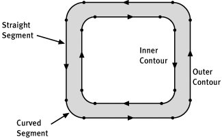
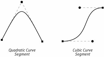
Chapter 3 discussed a drawing idiom that this book calls the Crayon Model. To briefly recap that idea, drawing line art with Quartz 2D involves outlining an area of user space and then either filling in that area or drawing a line that runs along its edge. Paths are the tools that you use both to outline an area before filling it and to define a line that you wish to stroke.

If you're using the Core Graphics APIs, paths are stored in instances of class with the rather unimaginative name CGPath. You can either construct a path using the methods of that opaque data type or by using the methods that a CGContext supplies for constructing its current path. With this API you can draw a path by storing it in the current path of a context and calling method on that context to effect the actual drawing.

If you are using the Cocoa frameworks, there is a Cocoa class called NSBezierPath you can use to create, store, and draw a path. In Cocoa, therefore, the path itself and not the graphics context becomes the primary interface for drawing.

The paths constructed through both these API are made from the same components. Exploration of building paths continues in this chapter by examining the components that go into creating a path and then by looking at some of the characteristics of the kinds of paths used in Quartz 2D that make them attractive for drawing.

Components of a Path

Consider the simple path shown in Figure 6.2. For this illustration we have filled the path with gray. Everywhere else, including the white area in the center of the rectangle is actually outside of the path. You might also say this path has a hole punched out of its center.

Figure 6.2. The Different parts of a Path

This particular path is made up of two subpaths, or contours. The first contour, labeled the Outer Contour in the figure, defines the outside edge of the path. The second contour, the Inner Contour, is the boundary of the rectangular hole in the center. Each of these contours is made up of a number of segments. The segments are the straight and curved lines between the dots on the figure. Labels point out one straight segment and one curved segment in the figure. Each contour in Figure 6.2 is made from eight segments.

Both contours are composite curves, that is, curves made up of smaller curves. The contours are created by chaining the end point of one segment onto the starting point of the next segment. This is precisely the way that a Quartz 2D application builds paths. Your application tells Quartz where to start the path and then adds curved segments, one after the other, to create a contour. After completing one contour, you tell Quartz 2D where to start the next contour and repeat the process.

The computer keeps track of the endpoint of the last segment you've added to the path you are working on, and this point becomes the starting place for the next segment. To continue that segment, you supply one or more new points. The number of points you have to supply to define a segment depends on the type of segment you want to add. Straight segments require you to supply only one point, the endpoint of the line. To create curved segments, however, you supply one or two intermediate points in addition to the endpoint. The computer uses these intermediate points to draw the curve, a bezier curve, that connects the two endpoints. Taken together the endpoints and the intermediate points are called the control points of the curve.

There is one more feature of the path contours illustrated in Figure 6.2. The order in which the application adds points to the contour imparts an intrinsic direction for that contour as well. The figure illustrates the direction of the contours with little arrowheads. The inner contour travels in a clockwise direction, and the outer contour turns counterclockwise. Contour directions can come into play when Quartz 2D is trying to determine what areas of the coordinate system are inside the path and which are outside. For more information on this, see the section on winding rules in the next chapter.

Bezier Curves

The technique of using bezier curves in computer graphics was pioneered by a gentleman named Pierre Bezier in the late 1960's. Mr. Bezier was a mathematician working for the Renault car company in France. Researchers at Renault were looking for a way to represent the curved surfaces that made up the bodies of their cars using mathematical techniques that were suitable for implementation on computers. Prior to that the curves were stored as unreliable hand-drawn sketches or as clay models. The result of that research was a simple, yet elegant mathematical model for representing curves that has become the foundation of many computer graphics technologies since.

Quartz 2D allows your application to use two different types of bezier curves as the segments of a path, quadratic and cubic. The terms quadratic and cubic refer to the degree of the mathematical equations that define the curve. For our purposes here, it is not important that we understand the mathematics of the equations involved, but we do need to understand the consequences of selecting one type of curve or the other. Rather than examine the mathematics of the curves, therefore, we look at them as design elements and discuss the advantages and disadvantages of each.

To begin our exploration we will look at individual curve segments and then expand that knowledge to encompass compound curves. Figure 6.3 illustrates both a quadratic and a cubic curve segment. In the figure, the curves themselves are the black lines. Each curve is annotated with small square markers that coincide with the endpoints of the segments. Also shown are small circular markers that denote the locations of additional points called bezier control points (BCPs). The BCPs, along with the endpoints, define the location and shape of the curve. The dashed gray lines connecting the BCPs to the endpoints help to illustrate how the BCPs affect the curve.

Figure 6.3. Bezier Curve Segment Types

Quadratic curves have only one BCP as illustrated in Figure 6.3. Cubic curves have two BCPs, one corresponding to each end of the curve. Your application shapes the curves by selecting the location of these control points.

You might think of it this way... from its the starting point, the curve starts out traveling along the straight line segment that connects the end point to the next BCP. However, as the curve moves along, the other BCPs (or the other end points) each draw the curve toward them in turn. By the end of the trip, the curve has reached the second endpoint. When it reaches the end, it is traveling in the direction of the line that joins the last BCP to the end point.

From this description, you might conclude that having more control points allows a curve to be more flexible. This is indeed the case. As you trace a quadratic curve from its start point to its ending point, there is only one BCP to attract the curve. That means that the curve is only allowed to bend once. The quadratic curve, in contrast, has two BCPs, and it can bend twice.

Mathematically, it is possible to create bezier curves in which a single curve bends as many times as you like. As you increase the number of control points in the segment, however, the calculations needed to draw the curve become very expensive. In addition, the intermediate control points of such a curve do not have the same intuitive relationship to the curve that the BCPs of quadratic and cubic curves have. Graphics libraries like Quartz 2D use quadratic and cubic curves because they strike a good balance between graphic flexibility and the cost of computing with them.

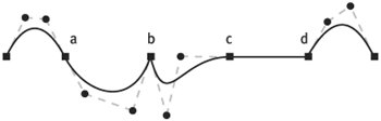
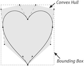
Because they contain fewer points, quadratic curves require less storage space for each segment than cubic segments. The mathematics of quadratic curves also involves a lot of dividing by two, which makes it easier for a computer to crunch the numbers as well. The greater flexibility of the cubic curve, however, means that it takes fewer cubic curves, on balance, to describe a complex shape.

Composite Curves

The path building routines in Quartz 2D focus on the task of creating a composite curve from individual quadratic and cubic segments. The segments join together simply by virtue of the fact that each bezier segment defines a curve that passes both endpoints. When you build a curve using a Quartz 2D method, the endpoint of one segment curve becomes the starting point of the next. This guarantees that the two segments will touch.

As you work with composite curves, the way that the joint between one segment and the next looks can be an important aspect of getting the drawing just right. Except in degenerate cases, the segments themselves are smooth curves. If you want sharp corners in your path, it is usually easier to locate the corner at the joint between two segments. By the same token, you might also want to ensure that the end of one segment flows smoothly into the next. All of these effects are controlled by the placement of the BCP handles on the segments on either side of the joint.

Figure 6.4 shows a compound curve constructed from cubic curve segments. It illustrates some of the techniques your application can use at the joints to achieve some common effects.

Figure 6.4. Different Ways of Joining Curve Segments

An interesting thing to note about Figure 6.4 is the addition of a line segment between the BCPs of each segment. The collection of line segments connecting the endpoints to the BCPs and the BCPs to each other forms a polygon called the control polygon.

The figure illustrates the joining points between four different curve segments. At point (a), the joint between the first two segments, the curve makes a smooth transition from one segment to the next. Notice that the last BCP of the first segment, the end point, and the first BCP of the second segment all lie in a straight line (they are colinear). Because the first segment ends on the line connecting the last BCP and the endpoint, and the second segment begins in the direction from the start point to the first BCP, when all these points line up, you get a smooth joint.

At point (b), the two curves meet because their endpoints coincide, but the BCPs on either side of the shared on-curve point are not colinear. The resulting curve shows a bend or discontinuity that forms a sharp cusp.

At point (c) the curve turns smoothly into the line because the control point to the left of the curve is colinear with the line. Lines are really just special cases of curves with the BCPs and the endpoints at the same location.

Finally, point (d) shows that the joint between a curve segment and a straight line need not be a smooth and orderly affair. This segment's first control point is not lined up with the previous segment, so the path draws with a slight corner at this joint.

Features of Bezier Curves

Bezier curves have some additional features that make them attractive for use in computer graphics. Mathematicians like to give these properties complex names, but the ideas behind them are pretty straightforward.

One of the primary benefits of bezier curves is the fact that they are smooth, continuous structures. A computer can take a bezier curve and break it into two or more segments that are also bezier curves. Mathematicians call this process subdivision, and it is an important feature of the curves that Quartz 2D exploits to provide the resolution independence of its line art.

Mathematicians also like to talk about the convex hull property of bezier curves. Basically what the convex hull property tells you is that a curve segment (and by extension a composite curve) will never go outside of the convex hull of its control polygon. An intuitive way to think about the convex hull of a set of points is to imagine putting little pegs in a board at each of the points and stretching a rubber band around the outermost pegs. The shape that the rubber band would form is the convex hull of the curve. Figure 6.5 shows the heart-shaped path from the Chapter 3 sample code with its control polygon and the convex hull of that polygon.

Figure 6.5. Heart-Shaped Path with Convex Hull and Bounding Box

The convex hull property makes it easy to find a bounding rectangle for a bezier curve. Because the curve is completely contained inside of its convex hull, any bounding rectangle of the convex hull is also a bounding rectangle of the curve. That bounding box might not be the smallest bounding box for the curve, but getting a more accurate box requires the computer to calculate points on the curve. Computing the bounds of the convex hull doesn't require any fancy math and is close enough for many applications. Figure 6.4 also illustrates the bounding box of the convex hull.

A third useful feature of bezier curves is what mathematicians call affine invariance. To cut a long story short, affine invariance means that if you want to transform a bezier curve using the kinds of transformations Quartz 2D supports, you can transform the points of the control polygon and then recompute the curve. If bezier curves did not have this property, then you could only transform the curve by calculating a number of points in the curve and transforming the larger set of points. Affine invariance allows the computer to efficiently apply Quartz 2D's affine transformations to curves.