| Previous | Table of Contents | Next |
Chapter 5
The Fundamentals of OSPF Routing & Design The Art of Strategy: “who are victorious plan effectively and change decisively. They are like a great river that maintains its course but adjusts its flow . . . they have form but are formless. They are skilled in both planning and adapting and need not fear the result of a thousand battles; for they win in advance, defeating those that have already lost.”—Sun Tzu, Chinese Warrior and Philosopher, 100 B.C. This chapter covers a variety of subjects all relating to routing and designing OSPF networks. The foundation laid in the previous chapters is further expanded as the discussion of OSPF performance and design issues is expanded. Within each of the design sections, a series of “golden design rules” is presented. These rules will help the reader understand the constraints and recommendations of properly designing each section of an overall OSPF network. In many cases, examples that draw upon the material are presented to further reinforce key topics and ideas. The author would like to recognize the previous works presented on OSPF routing and design done by Dennis Black and Bassam Halabi. Both gentlemen penned internal Cisco documents and have done a commendable job of presenting the OSPF-related material in an easy-to-understand format. This chapter is built from that framework. In some cases, the material is presented directly from the original text, but the majority of the information has been expanded upon. For additional information on the two sources used in this chapter, please see the bibliography. - • OSPF Algorithms. The OSPF algorithm will be discussed in greater detail with the introduction of costs. With the addition of costs, the routing tables of OSPF become altered, and this section explains how and why.
- • OSPF Convergence. This section covers the issues surrounding convergence with the protocol, including the benefits of OSPF and its ability to converge very quickly.
- • OSPF Design Guidelines. This section begins the introduction to design OSPF networks and concentrates on two main points: network topology and scalability. This section begins to examine the physical requirements and layout needed before the actual work begins.
- • Area Design Considerations. The true fundamentals of any OSPF network are its areas. The proper design of these areas is absolutely essential and the many different areas are discussed: backbone, non-stub, and all the variations of the stub area.
- • OSPF Route Selection. Routing is the essence of every protocol, and how the protocol determines its routes is the primary area of focus in this section. Included within this chapter is OSPF’s inherent capability to conduct load balancing. The derivation of external routes is also discussed at length.
- • OSPF IP Addressing & Route Summarization. General route summarization techniques and procedures used by OSPF are examined and demonstrated through several different scenarios that a network engineer may come into contact with. This section concludes with an in-depth discussion of VLSM and the benefits of its use in your OSPF network.
OSPF Algorithms OSPF is a link-state protocol that uses a link-state database (LSDB) in order to build and calculate the shortest path to all known destinations. It is through the use of the SPF algorithm that the information contained within the LSDB is calculated into routes. The shortest path algorithm by itself is quite complicated, and its inner workings are really beyond the scope of this book. But understanding its place and operation is essential to achieving a full understanding of OSPF. The text that follows reviews the operation of calculating the shortest path and then applies that to an example. The following is a very high level, simplified way of looking at the various steps used by the algorithm: - 1. Upon initialization or due to any change in routing information, a router will generate a link-state advertisement (LSA). This advertisement will represent the collection of all link-states on that router.
- 2. All routers will exchange LSAs by means of the OSPF Flooding protocol. Each router that receives a link-state update will store it in its LSDB and then flood the update to other routers.
- 3. After the database of each router is updated, each router will recalculate a shortest path tree to all destinations. The router uses the Shortest Path First (Dijkstra) algorithm to calculate the shortest path tree based on the LSDB. The destinations, their associated costs, and the next hop to reach those destinations will form the IP routing table.
The shortest path is calculated using the Dijkstra algorithm. The algorithm places each router at the root of a tree and calculates the shortest path to each destination based on the cumulative cost required to reach that destination. Each router will have its own view of the network’s topology even though all the routers will build a shortest path tree using the same LSDB. This view consists of what paths and their associated costs are available to reach destinations throughout the network. In Figure 5-1, the Headquarters router is at the base of the tree (turn figure upside down). The following sections indicate what is involved in building a shortest path tree. 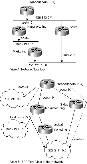
Figure 5-1 Shortest path cost calculation: How the network looks from the HQ router perspective.
OSPF Cost The cost or metric associated with an interface in OSPF is an indication of the overhead required to send packets across that interface. For example, in Figure 5-1, for Headquarters to reach network 192.213.11.0, a cost of 20 (10+5+5) is associated with the shortest path. The cost of an interface is inversely proportional to the bandwidth of that interface. A higher bandwidth indicates a lower cost. There is more overhead (higher cost) and time delays involved in crossing a 56K serial line than crossing a 10M Ethernet line. The formula used by OSPF to calculate the cost is - Cost=100,000,000/bandwith in bps
For example, it will cost 10 EXP8/10 EXP7=10 to cross a 10M Ethernet line and will cost 10 EXP8/1544000=64 to cross a T1 line. By default, the cost of an interface is calculated based on the bandwidth, but you can place a cost on an interface through the use of the ip ospf cost [value] interface command.
| Previous | Table of Contents | Next |
|