A Transportation Example
| The Zephyr Television Company ships televisions from three warehouses to three retail stores on a monthly basis. Each warehouse has a fixed supply per month, and each store has a fixed demand per month. The manufacturer wants to know the number of television sets to ship from each warehouse to each store in order to minimize the total cost of transportation. Each warehouse has the following supply of televisions available for shipment each month:
Each retail store has the following monthly demand for television sets:
Costs of transporting television sets from the warehouses to the retail stores vary as a result of differences in modes of transportation and distances. The shipping cost per television set for each route is as follows :
Decision VariablesThe model for this problem consists of nine decision variables, representing the number of television sets transported from each of the three warehouses to each of the three stores: x ij = number of television sets shipped from warehouse i to store j where i = 1, 2, 3, and j = A, B, C The variable x ij is referred to as a double-subscripted variable. The subscript, whether double or single, simply gives a " name " to the variable (i.e., distinguishes it from other decision variables). For example, the decision variable x 3A represents the number of television sets shipped from warehouse 3 in Pittsburgh to store A in New York. A double-subscripted variable is simply another form of variable name . The Objective FunctionThe objective function of the television manufacturer is to minimize the total transportation costs for all shipments. Thus, the objective function is the sum of the individual shipping costs from each warehouse to each store: minimize Z = $16 x 1A + 18 x 1B + 11 x 1C + 14 x 2A + 12 x 2B + 13 x 2C + 13 x 3A + 15 x 3B + 17 x 3C Model ConstraintsThe constraints in this model are the number of television sets available at each warehouse and the number of sets demanded at each store. There are six constraintsone for each warehouse's supply and one for each store's demand. For example, warehouse 1 in Cincinnati is able to supply 300 television sets to any of the three retail stores. Because the number shipped to the three stores is the sum of x 1A , x 1B , and x 1C , the constraint for warehouse 1 is x 1A + x 1B + x 1C This constraint is a x 2A + x 2B + x 2C x 3A + x 3B + x 3C In a "balanced" transportation model , supply equals demand such that all constraints are equalities; in an "unbalanced" transportation model , supply does not equal demand, and one set of constraints is The three demand constraints are developed in the same way as the supply constraints, except that the variables summed are the number of television sets supplied from each of the three warehouses. Thus, the number shipped to one store is the sum of the shipments from the three warehouses. They are equalities because all demands can be met: x 1A + x 2A + x 3A = 150 x 1B + x 2B + x 3B = 250 x 1C + x 2C + x 3C = 200 Model SummaryThe complete linear programming model for this problem is summarized as follows: minimize Z = $16 x 1A + 18 x 1B + 11 x 1C + 14 x 2A + 12 x 2B + 13 x 2C + 13 x 3A + 15 x 3B + 17 x 3C subject to Computer Solution with Excel The computer solution for this model was achieved using Excel and is shown in Exhibit 4.15. Notice that the objective function contained in cell C11 is shown on the formula bar at the top of the screen. The constraints for supply are included in cells F5, F6, and F7, whereas the demand constraints are in cells C8, D8, and E8. Thus, a typical supply constraint for Cincinnati would be C5+D5+E5 Exhibit 4.15.(This item is displayed on page 131 in the print version)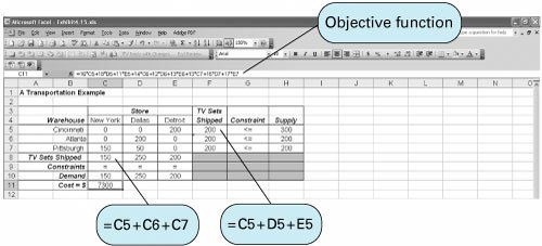 Exhibit 4.16.(This item is displayed on page 131 in the print version)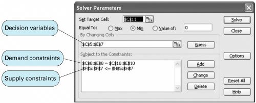 Solution AnalysisThe solution is x 1C = 200 TVs shipped from Cincinnati to Detroit x 2B = 200 TVs shipped from Atlanta to Dallas
Note that the surplus for the first constraint, which is the supply at the Cincinnati warehouse, equals 100 TVs. This means that 100 TVs are left in the Cincinnati warehouse, which has inventory and storage implications for the manager. This is an example of a type of linear programming model known as a transportation problem , which is the topic of Chapter 6. Notice that all the solution values are integer values. This is always the case with transportation problems because of the unique characteristic that all the coefficient parameter values are ones and zeros. | |||||||||||||||||||||||||||||||||||||||||||||||||
 300
300 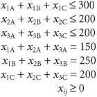
EAN: 2147483647
Pages: 358