Computer Solution
| When linear programming was first developed in the 1940s, virtually the only way to solve a problem was by using a lengthy manual mathematical solution procedure called the simplex method . However, during the next six decades, as computer technology evolved, the computer was used more and more to solve linear programming models. The mathematical steps of the simplex method were simply programmed in prewritten software packages designed for the solution of linear programming problems. The ability to solve linear programming problems quickly and cheaply on the computer, regardless of the size of the problem, popularized linear programming and expanded its use by businesses. There are currently dozens of software packages with linear programming capabilities. Many of these are general-purpose management science or quantitative methods packages with linear programming modules, among many other modules for other techniques. There are also numerous software packages that are devoted exclusively to linear programming and its derivatives. These packages are generally cheap, efficient, and easy to use. The simplex method is a procedure involving a set of mathematical steps to solve linear programming problems. As a result of the easy and low-cost availability of personal computers and linear programming software, the simplex method has become less of a focus in the teaching of linear programming. Thus, at this point in our presentation of linear programming, we focus exclusively on computer solution. However, knowledge of the simplex method is useful in gaining an overall, in-depth understanding of linear programming for those who are interested in this degree of understanding. As noted, computer solution itself is based on the simplex method. Thus, while we present linear programming in the text in a manner that does not require use of the simplex method, we also provide in-depth coverage of this topic on the CD that accompanies this text. In the next few sections we demonstrate how to solve linear programming problems by using Excel spreadsheets and QM for Windows , a typical general-purpose quantitative methods software package. Excel SpreadsheetsExcel can be used to solve linear programming problems, although the data input requirements can be more time-consuming and tedious than with a software package like QM for Windows that is specifically designed for the purpose. A spreadsheet requires that column and row headings for the specific model be set up and that constraint and objective function formulas be input in their entirety, as opposed to just the model parameters, as with QM for Windows. However, this is also an advantage of spreadsheets, in that it enables the problem to be set up in an attractive format for reporting and presentation purposes. In addition, once a spreadsheet is set up for one problem, it can often be used as a template for others. Exhibit 3.1 shows an Excel spreadsheet set up for our Beaver Creek Pottery Company example introduced in Chapter 2. Appendix B at the end of this text is the tutorial "Setting Up and Editing a Spreadsheet," using Exhibit 3.5 as an example. Exhibit 3.1.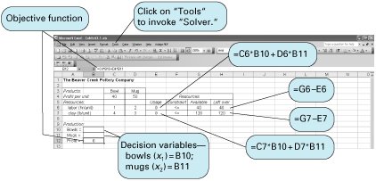 The values for bowls and mugs and for profit are contained in cells B10, B11, and B12, respectively. These cells are currently empty because the model has not yet been solved . The objective function for profit, = C4*B10+D4*B11 , is embedded in cell B12 and shown on the formula bar at the top of the screen. This formula is essentially the same as Z = 40 x 1 + 50 x 2 , where B10 and B11 represent x 1 and x 2 , and B12 equals Z . The objective function coefficients, 40 and 50, are in cells C4 and D4. Similar formulas for the constraints for labor and clay are embedded in cells E6 and E7. For example, in cell E6 we input the formula = C6*B10+D6*B11 . The <= signs in cells F6 and F7 are for cosmetic purposes only; they have no real effect. To solve this problem, first bring down the "Tools" menu from the toolbar at the top of the screen and then select "Solver" from the list of menu items. (If "Solver" is not shown on the "Tools" menu, then it can be activated by clicking on "Add-ins" on the "Tools" menu and then "Solver." If Solver is not available from the "Add-ins" menu, it must be installed on the "Add-ins" menu directly from your Office or Excel software. For example, in Office you would access "Office Setup," then the "Office Applications" menu, then "Excel," then "Add-ins," and then activate "Solver.") The window Solver Parameters will appear, as shown in Exhibit 3.2. Initially all the windows on this screen are blank, and we must input the objective function cell, the cells representing the decision variables , and the cells that make up the model constraints. Exhibit 3.2.(This item is displayed on page 74 in the print version)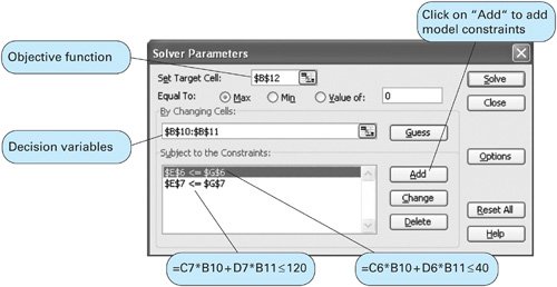 When inputting the Solver parameters as shown in Exhibit 3.2, we first input the "target cell" that contains our objective function, which is B12 for our example. (Excel automatically inserts the $ sign next to cell addresses; you should not type it in.) Next we indicate that we want to maximize the target cell by clicking on "Max." We achieve our objective by changing cells B10 and B11, which represent our model decision variables. The designation "B10:B11" means all the cells between B10 and B11, inclusive. We next input our model constraints by clicking on "Add," which will access the screen shown in Exhibit 3.3. Exhibit 3.3.(This item is displayed on page 74 in the print version)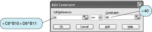 Exhibit 3.3 shows our labor constraint. Cell E6 contains the constraint formula for labor (= C6*B10+D6*B11 ), whereas cell G6 contains the labor hours available (i.e., 40). We continue to add constraints until the model is complete. Note that we could have input our constraints by adding a single constraint formula, E6:E7 <= G6:G7 , which means that the constraints in cells E6 and E7 are less than or equal to the values in cells G6 and G7, respectively. It is also not necessary to input the nonnegativity constraints for our decision variables, B10:B11 >= . This can be achieved in the Options screen, as explained next. Click on "OK" on the Add Constraint window after all constraints have been added. This will return us to the Solver Parameters screen. There is one more necessary step before proceeding to solve the problem. Select "Options" from the Solver Parameters screen and then when the Options screen appears, as shown in Exhibit 3.4, click on "Assume Linear Models." This will ensure that Solver uses the simplex procedure to solve the model and not some other numeric method (which Excel has available). This is not too important for now, but later it will ensure that we get the right reports for sensitivity analysis, a topic we will take up next. Notice that the Options screen also enables you to establish the nonnegativity conditions by clicking on "Assume Non-Negative." Click on "OK" to return to Solver. Exhibit 3.4.(This item is displayed on page 75 in the print version)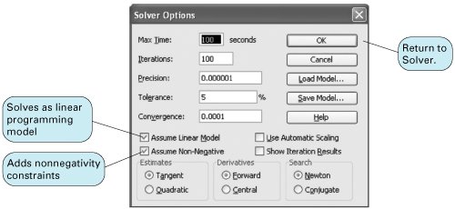 Once the complete model is input, click on "Solve" in the upper-right corner of the Solver Parameters screen (Exhibit 3.2). First, a screen will appear, titled Solver Results, which will provide you with the opportunity to select the reports you want and then when you click on "OK," the solution screen shown in Exhibit 3.5 will appear. Exhibit 3.5.(This item is displayed on page 75 in the print version)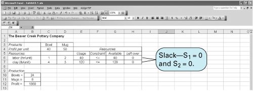 If there had been any extra, or slack , left over for labor or clay, it would have appeared in column H on our spreadsheet, under the heading "Left Over." In this case there are no slack resources left over. We can also generate several reports that summarize the model results. When you click on "OK" from the Solver screen, an intermediate screen will appear before the original spreadsheet, with the solution results. This screen is titled Solver Results, and it provides an opportunity for you to select several reports, including the answer report, shown in Exhibit 3.6. This report provides a summary of the solution results. Exhibit 3.6.(This item is displayed on page 76 in the print version)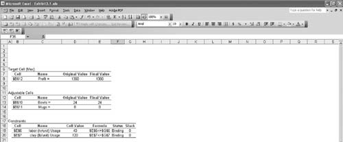 QM for WindowsBefore demonstrating how to use QM for Windows, we must first make a few comments about the proper form that constraints must be in before a linear programming model can be solved with QM for Windows. The constraints formulated in the linear programming models presented in Chapter 2 and in this chapter have followed a consistent form. All the variables in the constraint have appeared to the left of the inequality, and all numerical values have been on the right-hand side of the inequality. For example, in the pottery company model, the constraint for labor is x 1 + 2 x 2 The value, 40, is referred to as the constraint quantity, or right-hand-side , value. The standard form for a linear programming problem requires constraints to be in this form, with variables on the left side and numeric values to the right of the inequality or equality sign. This is a necessary condition to input problems into some computer programs, and specifically QM for Windows, for linear programming solution.
Consider a model requirement which states that the production of product 3 ( x 3 ) must be as much as or more than the production of products 1 ( x 1 ) and 2 ( x 2 ). The model constraint for this requirement is formulated as x 3 This constraint is not in proper form and could not be input into QM for Windows as it is. It must first be converted to x 3 x 1 x 2 This constraint can now be input for computer solution. Next consider a problem requirement that the ratio of the production of product 1 ( x 1 ) to the production of products 2 ( x 2 ) and 3 ( x 3 ) must be at least 2 to 1. The model constraint for this requirement is formulated as Although this constraint does meet the condition that variables be on the left side of the inequality and numeric values on the right, it is not in proper form. The fractional relationship of the variables, x 1 /( x 2 + x 3 ), cannot be input into the most commonly used linear programming computer programs in that form. It must be converted to x 1 and x 1 - 2 x 2 - 2 x 3 Fractional relationships between variables in constraints must be eliminated. We will demonstrate how to use QM for Windows by solving our Beaver Creek Pottery Company example. The linear programming module in QM for Windows is accessed by clicking on "Module" at the top of the initial window. This will bring down a menu with all the program modules available in QM for Windows, as shown in Exhibit 3.7. By clicking on "Linear Programming," a window for this program will come up on the screen, and by clicking on "File" and then "New," a screen for inputting problem dimensions will appear. Exhibit 3.8 shows the data entry screen with the model type and the number of constraints and decision variables for our Beaver Creek Pottery Company example. Exhibit 3.7.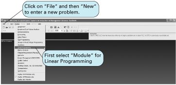 Exhibit 3.8.(This item is displayed on page 78 in the print version)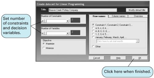 Exhibit 3.9 shows the data table for our example, with the model parameters, including the objective function and constraint coefficients, and the constraint quantity values. Notice that we also customized the row headings for the constraints by typing in "Labor (hrs)" and "Clay (lbs)." Once the model parameters have been input, click on "Solve" to get the model solution, as shown in Exhibit 3.10. It is not necessary to put the model into standard form by adding slack variables. Exhibit 3.9.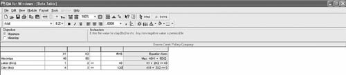 Exhibit 3.10.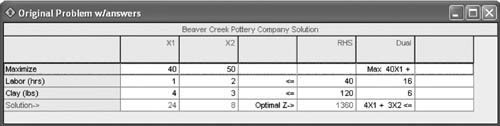 The marginal value is the dollar amount one would be willing to pay for one additional resource unit. Notice the values 16 and 6 under the column labeled "Dual" for the "Labor" and "Clay" rows. These dual values are the marginal values of labor and clay in our problem. This is useful information that is provided in addition to the normal model solution values when you solve a linear programming model. We talk about dual values in more detail later in this chapter, but for now it is sufficient to say that the marginal value is the dollar amount the company would be willing to pay for one additional unit of a resource. For example, the dual value of 16 for the labor constraint means that if 1 additional hour of labor could be obtained by the company, it would increase profit by $16. Likewise, if 1 additional pound of clay could be obtained, it would increase profit by $6. Thus, the company would be willing to pay up to $16 for 1 more hour of labor and $6 for 1 more pound of clay. The dual value is not the purchase price of one of these resources; it is the maximum amount the company would pay to get more of the resource. These dual values are helpful to the company in making decisions about acquiring additional resources. QM for Windows provides solution results in several different formats, including a graphical solution by clicking on "Window" and then selecting "Graph." Exhibit 3.11 shows the graphical solution for our Beaver Creek Pottery Company example. Exhibit 3.11.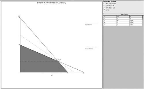 |
 40
40 

EAN: 2147483647
Pages: 358