Solution of the Transportation Model
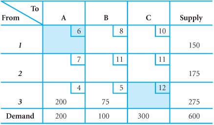
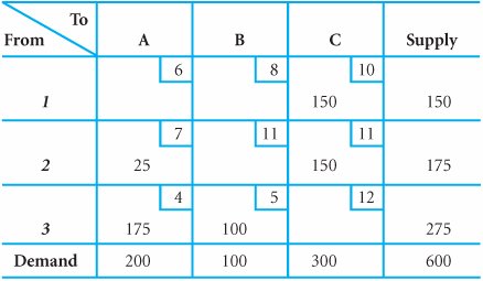
| The following example was used in chapter 6 of the text to demonstrate the formulation of the transportation model. Wheat is harvested in the Midwest and stored in grain elevators in three different citiesKansas City, Omaha, and Des Moines. These grain elevators supply three flour mills, located in Chicago, St. Louis, and Cincinnati. Grain is shipped to the mills in railroad cars, each car capable of holding one ton of wheat. Each grain elevator is able to supply the following number of tons (i.e., railroad cars ) of wheat to the mills on a monthly basis.
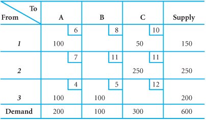
Each mill demands the following number of tons of wheat per month.
The cost of transporting one ton of wheat from each grain elevator (source) to each mill (destination) differs according to the distance and rail system. These costs are shown in the following table. For example, the cost of shipping one ton of wheat from the grain elevator at Omaha to the mill at Chicago is $7.
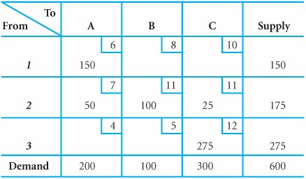
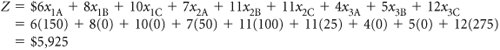
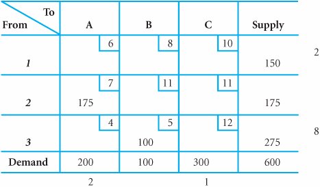
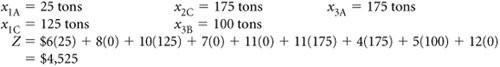
The problem is to determine how many tons of wheat to transport from each grain elevatorto each mill on a monthly basis in order to minimize the total cost of transportation. The linear programming model for this problem is formulated in the equations that follow. minimize Z = $6 x 1A + 8 x 1B + 10 x 1C + 7 x 2A + 11 x 2B + 11 x 2C + 4 x 3A + 5 x 3B + 12 x 3C subject to x 1A + x 1B + x 1C = 150 x 2A + x 2B + x 2C = 175 x 3A + x 3B + x 3C = 275 x 1A + x 2A + x 3A = 200 x 1B + x 2B + x 3B = 100 x 1C + x 2C + x 3C = 300 x ij In this model the decision variables , x ij , represent the number of tons of wheat transported from each grain elevator, i (where i = 1, 2, 3), to each mill, j (where j = A, B, C). The objective function represents the total transportation cost for each route. Each term in the objective function reflects the cost of the tonnage transported for one route. For example, if 20 tons are transported from elevator 1 to mill A, the cost of $6 is multiplied by x 1A (= 20), which equals $120. The first three constraints in the linear programming model represent the supply at each elevator; the last three constraints represent the demand at each mill. As an example, consider the first supply constraint, x 1A + x 1B + x 1C = 150. This constraint represents the tons of wheat transported from Kansas City to all three mills: Chicago ( x 1A ), St. Louis ( x 1B ), and Cincinnati ( x 1C ). The amount transported from Kansas City is limited to the 150 tons available. Note that this constraint (as well as all others) is an equation ( = ) rather than a Transportation problems are solved manually within a tableau format . Transportation models are solved manually within the context of a tableau , as in the simplex method. The tableau for our wheat transportation model is shown in Table B-1. Table B-1. The Transportation Tableau Each cell in the tableau represents the amount transported from one source to one destination. Thus, the amount placed in each cell is the value of a decision variable for that cell. For example, the cell at the intersection of row 1 and column A represents the decision variable x 1A . The smaller box within each cell contains the unit transportation cost for that route. For example, in cell 1A the value, $6, is the cost of transporting one ton of wheat from Kansas City to Chicago. Along the outer rim of the tableau are the supply and demand constraint quantity values, which are referred to as rim requirements . Each cell in a transportation tableau is analogous to a decision variable that indicates the amount allocated from a source to a destination. The supply and demand values along the outside rim of a tableau are called rim requirements . The two methods for solving a transportation model are the stepping-stone method and the modified distribution method (also known as MODI). In applying the simplex method, an initial solution had to be established in the initial simplex tableau. This same condition must be met in solving a transportation model. In a transportation model, an initial feasible solution can be found by several alternative methods, including the northwest corner method , the minimum cell cost method , and Vogel's approximation model . Transportation models do not start at the origin where all decision variables equal zero; they must be given an initial feasible solution . The Northwest Corner MethodWith the northwest corner method, an initial allocation is made to the cell in the upper lefthand corner of the tableau (i.e., the "northwest corner"). The amount allocated is the most possible, subject to the supply and demand constraints for that cell. In our example, we first allocate as much as possible to cell 1A (the northwest corner). This amount is 150 tons, since that is the maximum that can be supplied by grain elevator 1 at Kansas City, even though 200 tons are demanded by mill A at Chicago. This initial allocation is shown in Table B-2. Table B-2. The Initial NW Corner Solution In the northwest corner method the largest possible allocation is made to the cell in the upper left-hand corner of the tableau, followed by allocations to adjacent feasible cells . We next allocate to a cell adjacent to cell 1A, in this case either cell 2A or cell 1B. However, cell 1B no longer represents a feasible allocation, because the total tonnage of wheat available at source 1 (i.e., 150 tons) has already been allocated. Thus, cell 2A represents the only feasible alternative, and as much as possible is allocated to this cell. The amount allocated at 2A can be either 175 tons, the supply available from source 2 (Omaha), or 50 tons, the amount now demanded at destination A. (Recall that 150 of the 200 tons demanded at A have already been supplied.) Because 50 tons is the most constrained amount, it is allocated to cell 2A, as shown in Table B-2. The third allocation is made in the same way as the second allocation. The only feasible cell adjacent to cell 2A is cell 2B. The most that can be allocated is either 100 tons (the amount demanded at mill B) or 125 tons (175 tons minus the 50 tons allocated to cell 2A). The smaller (most constrained) amount, 100 tons, is allocated to cell 2B, as shown in Table B-2. The fourth allocation is 25 tons to cell 2C, and the fifth allocation is 275 tons to cell 3C, both of which are shown in Table B-2. Notice that all of the row and column allocations add up to the appropriate rim requirements. The initial solution is complete when all rim requirements are satisfied. The transportation cost of this solution is computed by substituting the cell allocations (i.e., the amounts transported), x 1A = 150 x 2A = 50 x 2B = 100 x 2C = 25 x 3C = 275 into the objective function. The steps of the northwest corner method are summarized here.
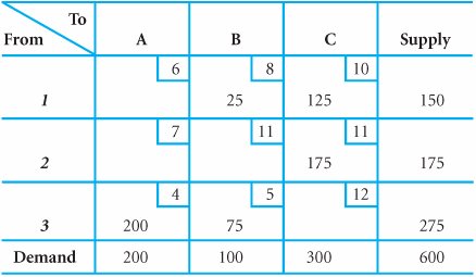
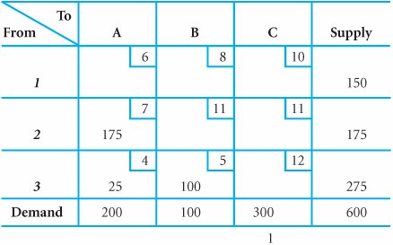
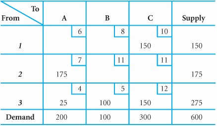
The Minimum Cell Cost MethodWith the minimum cell cost method, the basic logic is to allocate to the cells with the lowest costs. The initial allocation is made to the cell in the tableau having the lowest cost. In the transportation tableau for our example problem, cell 3A has the minimum cost of $4. As much as possible is allocated to this cell; the choice is either 200 tons or 275 tons. Even though 275 tons could be supplied to cell 3A, the most we can allocate is 200 tons, since only 200 tons are demanded. This allocation is shown in Table B-3. Table B-3. The Initial Minimum Cell Cost Allocation In the minimum cell cost method as much as possible is allocated to the cell with the minimum cost. Notice that all of the remaining cells in column A have now been eliminated, because all of the wheat demanded at destination A, Chicago, has now been supplied by source 3, Des Moines. The next allocation is made to the cell that has the minimum cost and also is feasible. This is cell 3B which has a cost of $5. The most that can be allocated is 75 tons (275 tons minus the 200 tons already supplied). This allocation is shown in Table B-4. Table B-4. The Second Minimum Cell Cost Allocation(This item is displayed on page B-6 in the print version) The third allocation is made to cell 1B, which has the minimum cost of $8. (Notice that cells with lower costs, such as 1A and 2A, are not considered because they were previously ruled out as infeasible.) The amount allocated is 25 tons. The fourth allocation of 125 tons is made to cell 1C, and the last allocation of 175 tons is made to cell 2C. These allocations, which complete the initial minimum cell cost solution, are shown in Table B-5. Table B-5. The Initial Solution The total cost of this initial solution is $4,550, as compared to a total cost of $5,925 for the initial northwest corner solution. It is not a coincidence that a lower total cost is derived using the minimum cell cost method; it is a logical occurrence. The northwest corner method does not consider cost at all in making allocationsthe minimum cell cost method does. It is therefore quite natural that a lower initial cost will be attained using the latter method. Thus, the initial solution achieved by using the minimum cell cost method is usually better in that, because it has a lower cost, it is closer to the optimal solution; fewer subsequent iterations will be required to achieve the optimal solution. The minimum cell cost method will provide a solution with a lower cost than the northwest corner solution because it considers cost in the allocation process . The specific steps of the minimum cell cost method are summarized next.
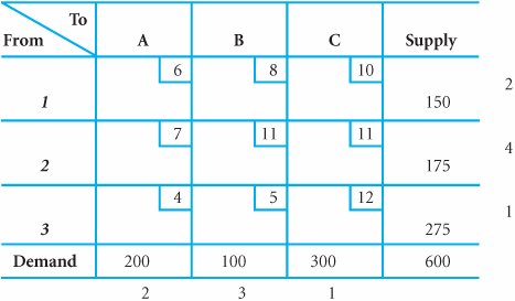
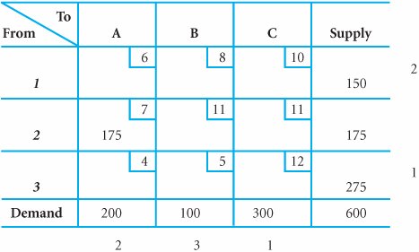
Vogel's Approximation ModelThe third method for determining an initial solution, Vogel's approximation model (also called VAM), is based on the concept of penalty cost or regret . If a decision maker incorrectly chooses from several alternative courses of action, a penalty may be suffered (and the decision maker may regret the decision that was made). In a transportation problem, the courses of action are the alternative routes, and a wrong decision is allocating to a cell that does not contain the lowest cost. A penalty cost is the difference between the largest and next largest cell cost in a row (or column) . In the VAM method, the first step is to develop a penalty cost for each source and destination. For example, consider column A in Table B-6. Destination A, Chicago, can be supplied by Kansas City, Omaha, and Des Moines. The best decision would be to supply Chicago from source 3 because cell 3A has the minimum cost of $4. If a wrong decision were made and the next higher cost of $6 were selected at cell 1A, a "penalty" of $2 per ton would result (i.e., $6 - 4 = $2). This demonstrates how the penalty cost is determined for each row and column of the tableau. The general rule for computing a penalty cost is to subtract the minimum cell cost from the next higher cell cost in each row and column. The penalty costs for our example are shown at the right and at the bottom of Table B-6. Table B-6. The VAM Penalty Costs VAM allocates as much as possible to the minimum cost cell in the row or column with the largest penalty cost . The initial allocation in the VAM method is made in the row or column that has the highest penalty cost. In Table B-6, row 2 has the highest penalty cost of $4. We allocate as much as possible to the feasible cell in this row with the minimum cost. In row 2, cell 2A has the lowest cost of $7, and the most that can be allocated to cell 2A is 175 tons. With this allocation the greatest penalty cost of $4 has been avoided because the best course of action has been selected. The allocation is shown in Table B-7. Table B-7. The Initial VAM Allocation After the initial allocation is made, all of the penalty costs must be recomputed. In some allocacases the penalty costs will change or be eliminated; in other cases they will not change. For example, the penalty cost in row 2 was eliminated altogether (because no more allocations are possible for that row). After each VAM cell allocation, all row and column penalty costs are recomputed Next, we repeat the previous step and allocate to the row or column with the highest penalty cost, which is now column B with a penalty cost of $3 (see Table B-7). The cell in column B with the lowest cost is 3B, and we allocate as much as possible to this cell, 100 tons. This allocation is shown in Table B-8. Table B-8. The Second VAM Allocation Note that all penalty costs have been recomputed in Table B-8. Since the highest penalty cost is now $8 for row 3 and since cell 3A has the minimum cost of $4, we allocate 25 tons to this cell, as shown in Table B-9. Table B-9. The Third VAM Allocation Table B-9 also shows the recomputed penalty costs after the third allocation. Notice that by now only column C has a penalty cost. Rows 1 and 3 have only one feasible cell, so a penalty does not exist for these rows. Thus, the last two allocations are made to column C. First, 150 tons are allocated to cell 1C because it has the lowest cell cost. This leaves only cell 3C as a feasible possibility, so 150 tons are allocated to this cell. Both of these allocations are shown in Table B-10. Table B-10. The Initial VAM Solution(This item is displayed on page B-9 in the print version) The total cost of this initial Vogel's approximation model solution is $5,125, which is not as high as the northwest corner initial solution of $5,925. It is also not as low as the minimum cell cost solution of $4,550. Like the minimum cell cost method, VAM typically results in a lower cost for the initial solution than does the northwest corner method. VAM and minimum cell cost both provide better initial solutions than the northwest corner method The steps of Vogel's approximation model can be summarized in the following list.
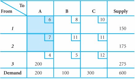
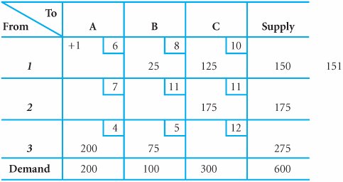
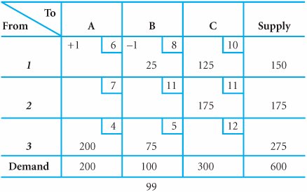
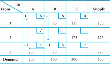
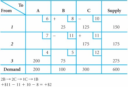
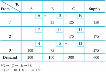
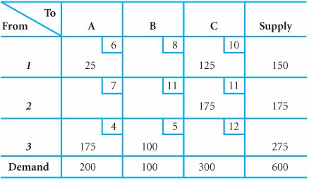
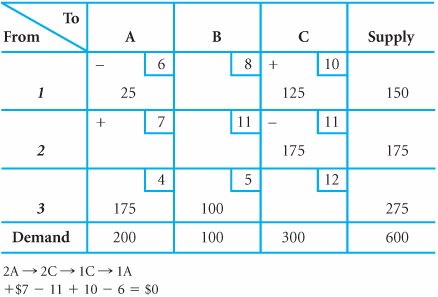
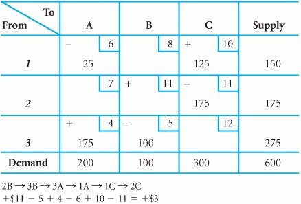
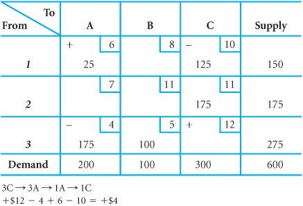
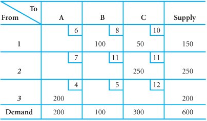
The Stepping-Stone Solution MethodOnce an initial basic feasible solution has been determined by any of the previous three methods, the next step is to solve the model for the optimal (i.e., minimum total cost) solution. There are two basic solution methods: the stepping-stone solution method and the modified distribution method (MODI). The stepping-stone solution method will be demonstrated first. Because the initial solution obtained by the minimum cell cost method had the lowest total cost of the three initial solutions, we will use it as the starting solution. Table B-11 repeats the initial solution that was developed from the minimum cell cost method. Table B-11. The Minimum Cell Cost Solution Once an initial solution is derived, the problem must be solved using either the stepping-stone method or MODI . The basic solution principle in a transportation problem is to determine whether a transportation route not at present being used (i.e., an empty cell) would result in a lower total cost if it were used. For example, Table B-11 shows four empty cells (1A, 2A, 2B, 3C) representing unused routes. Our first step in the stepping-stone method is to evaluate these empty cells to see whether the use of any of them would reduce total cost. If we find such a route, then we will allocate as much as possible to it. The stepping-stone method determines if there is a cell with no allocation that would reduce cost if used . First, let us consider allocating one ton of wheat to cell 1A. If one ton is allocated to cell 1A, cost will be increased by $6the transportation cost for cell 1A. However, by allocating one ton to cell 1A, we increase the supply in row 1 to 151 tons, as shown in Table B-12. Table B-12. The Allocation of One Ton to Cell 1A The constraints of the problem cannot be violated, and feasibility must be maintained . If we add one ton to cell 1A, we must subtract one ton from another allocation along that row. Cell 1B is a logical candidate because it contains 25 tons. By subtracting one ton from cell 1B, we now have 150 tons in row 1, and we have satisfied the supply constraint again. At the same time, subtracting one ton from cell 1B has reduced total cost by $8. However, by subtracting one ton from cell 1B, we now have only 99 tons allocated to column B, where 100 tons are demanded, as shown in Table B-13. To compensate for this constraint violation, one ton must be added to a cell that already has an allocation . Since cell 3B has 75 tons, we will add one ton to this cell, which again satisfies the demand constraint of 100 tons. Table B-13. The Subtraction of One Ton from Cell 1B A requirement of this solution method is that units can only be added to and subtracted from cells that already have allocations. That is why one ton was added to cell 3B and not to cell 2B. It is from this requirement that the method derives its name . The process of adding and subtracting units from allocated cells is analogous to crossing a pond by stepping on stones (i.e., only allocated-to cells). By allocating one extra ton to cell 3B we have increased cost by $5, the transportation cost for that cell. However, we have also increased the supply in row 3 to 276 tons, a violation of the supply constraint for this source. As before, this violation can be remedied by subtracting one ton from cell 3A, which contains an allocation of 200 tons. This satisfies the supply constraint again for row 3, and it also reduces the total cost by $4, the transportation cost for cell 3A. These allocations and deletions are shown in Table B-14. Table B-14. The Addition of One Ton to Cell 3B and the Subtraction of One Ton from Cell 3A Notice in Table B-14 that by subtracting one ton from cell 3A, we did not violate the demand constraint for column A, since we previously added one ton to cell 1A. Now let us review the increases and reductions in costs resulting from this process. We initially increased cost by $6 at cell 1A, then reduced cost by $8 at cell 1B, then increased cost by $5 at cell 3B, and, finally, reduced cost by $4 at cell 3A. In other words, for each ton allocated to cell 1A (a route not at present used), total cost will be reduced by $1. This indicates that the initial solution is not optimal because a lower cost can be achieved by allocating additional tons of wheat to cell 1A (i.e., cell 1A is analogous to a pivot column in the simplex method). Our goal is to determine the cell or entering "variable" that will reduce cost the most. Another variable (empty cell) may result in an even greater decrease in cost than cell 1A. If such a cell exists, it will be selected as the entering variable; if not, cell 1A will be selected. To identify the appropriate entering variable, the remaining empty cells must be tested as cell 1A was. An empty cell that will reduce cost is a potential entering variable . Before testing the remaining empty cells, let us identify a few of the general characteristics of the stepping-stone process. First, we always start with an empty cell and form a closed path of cells that now have allocations. In developing the path, it is possible to skip over both unused and used cells. In any row or column there can be only one addition and one subtraction. (For example, in row 1, wheat is added at cell 1A and is subtracted at cell 1B.) To evaluate the cost reduction potential of an empty cell, a closed path connecting used cells to the empty cell is identified . Let us test cell 2A to see if it results in a cost reduction. The stepping-stone closed path for cell 2A is shown in Table B-15. Notice that the path for cell 2A is slightly more complex than the path for cell 1A. Notice also that the path crosses itself at one point, which is perfectly acceptable. An allocation to cell 2A will reduce cost by $1, as shown in the computation in Table B-15. Thus, we have located another possible entering variable, although it is no better than cell 1A. Table B-15. The Stepping-Stone Path for Cell 2A(This item is displayed on page B-12 in the print version) The remaining stepping-stone paths and the resulting computations for cells 2B and 3C are shown in Tables B-16 and B-17, respectively. Table B-16. The Stepping-Stone Path for Cell 2B Table B-17. The Stepping-Stone Path for Cell 3C Notice that after all four unused routes are evaluated, there is a tie for the entering variable between cells 1A and 2A. Both show a reduction in cost of $1 per ton allocated to that route. The tie can be broken arbitrarily. We will select cell 1A (i.e., x 1A ) to enter the solution. After all empty cells are evaluated, the one with the greatest cost reduction potential is the entering variable . Because the total cost of the model will be reduced by $1 for each ton we can reallocate to cell 1A, we naturally want to reallocate as much as possible. To determine how much to allocate, we need to look at the path for cell 1A again, as shown in Table B-18. Table B-18. The Stepping-Stone Path for Cell 1A The stepping-stone path in Table B-18 shows that tons of wheat must be subtracted at cells 1B and 3A to meet the rim requirements and thus satisfy the model constraints. Because we cannot subtract more than is available in a cell, we are limited by the 25 tons in cell 1B. In other words, if we allocate more than 25 tons to cell 1A, then we must subtract more than 25 tons from 1B, which is impossible because only 25 tons are available. Therefore, 25 tons is the amount we reallocate to cell 1A according to our path. That is, 25 tons are added to 1A, subtracted from 1B, added to 3B, and subtracted from 3A. This reallocation is shown in Table B-19. Table B-19. The Second Iteration of the Stepping-Stone Method When reallocating units to the entering variable (cell), the amount is the minimum amount subtracted on the stepping-stone path . The process culminating in Table B-19 represents one iteration of the stepping-stone method. We selected x 1A as the entering variable, and it turned out that x 1B was the leaving variable (because it now has a value of zero in Table B-19). Thus, at each iteration one variable enters and one leaves (just as in the simplex method). Now we must check to see whether the solution shown in Table B-19 is, in fact, optimal. We do this by plotting the paths for the unused routes (i.e., empty cells 2A, 1B, 2B, and 3C) that are shown in Table B-19. These paths are shown in Tables B-20 through B-23. Table B-20. The Stepping-Stone Path for Cell 2A Table B-21. The Stepping-Stone Path for Cell 1B Table B-22. The Stepping-Stone Path for Cell 2B Table B-23. The Stepping-Stone Path for Cell 3C Our evaluation of the four paths indicates no cost reductions; therefore, the solution shown in Table B-19 is optimal. The solution and total minimum cost are The stepping-stone process is repeated until none of the empty cells will reduce cost (i.e., an optimal solution) . However, notice in Table B-20 that the path for cell 2A resulted in a cost change of $0. In other words, allocating to this cell would neither increase nor decrease total cost. This situation indicates that the problem has multiple optimal solutions of the text. Thus, x 2A could be entered into the solution and there would not be a change in the total minimum cost of $4,525. To identify the alternative solution, we would allocate as much as possible to cell 2A, which in this case is 25 tons of wheat. The alternative solution is shown in Table B-24. Table B-24. The Alternative Optimal Solution A multiple optimal solution occurs when an empty cell has a cost change of zero and all other empty cells are positive . An alternate optimal solution is determined by allocating to the empty cell with a zero cost change . The solution in Table B-24 also results in a total minimum cost of $4,525. The steps of the stepping-stone method are summarized here.
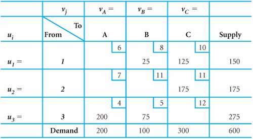
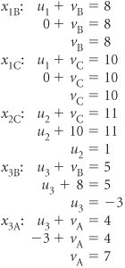
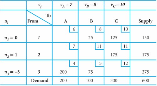
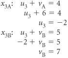
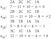
The Modified Distribution MethodThe modified distribution method (MODI) is basically a modified version of the steppingstone method. However, in the MODI method the individual cell cost changes are determined mathematically, without identifying all of the stepping-stone paths for the empty cells. To demonstrate MODI , we will again use the initial solution obtained by the minimum cell cost method. The tableau for the initial solution with the modifications required by MODI is shown in Table B-25. Table B-25. The Minimum Cell Cost Initial Solution MODI is a modified version of the stepping-stone method in which math equations replace the stepping-stone paths . The extra left-hand column with the u i symbols and the extra top row with the v j symbols represent column and row values that must be computed in MODI . These values are computed for all cells with allocations by using the following formula. u i + v j = c ij The value c ij is the unit transportation cost for cell ij . For example, the formula for cell 1B is u 1 + v B = c 1B and, since c 1B = 8, u 1 + v B = 8 The formulas for the remaining cells that presently contain allocations are
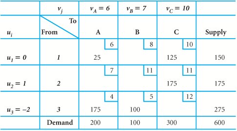
Now there are five equations with six unknowns. To solve these equations, it is necessary to assign only one of the unknowns a value of zero. Thus, if we let u 1 = 0, we can solve for all remaining u i and v j values. Notice that the equation for cell 3B had to be solved before the cell 3A equation could be solved. Now all the u i and v j values can be substituted into the tableau, as shown in Table B-26. Table B-26. The Initial Solution with All u i and v j Values Next, we use the following formula to evaluate all empty cells : c ij u i v j = k ij where k ij equals the cost increase or decrease that would occur by allocating to a cell. For the empty cells in Table B-26, the formula yields the following values:
These calculations indicate that either cell 1A or cell 2A will decrease cost by $1 per allocated ton. Notice that those are exactly the same cost changes for all four empty cells as were computed in the stepping-stone method. That is, the same information is obtained by evaluating the paths in the stepping-stone method and by using the mathematical formulas of the MODI. Each MODI allocation replicates the stepping-stone allocation . We can select either cell 1A or 2A to allocate to because they are tied at 1. If cell 1A is selected as the entering nonbasic variable, then the stepping-stone path for that cell must be determined so that we know how much to reallocate. This is the same path previously identified in Table B-18. Reallocating along this path results in the tableau shown in Table B-27 (and previously shown in Table B-19). Table B-27. The Second Iteration of the MODI Solution Method(This item is displayed on page B-18 in the print version) After each allocation to an empty cell, the u i and v j values must be recomputed . The u i and v j values for Table B-27 must now be recomputed using our formula for the allocated-to cells. These new u i and v j values are shown in Table B-28. Table B-28. The New u i and v j Values for the Second Iteration The cost changes for the empty cells are now computed using the formula c ij u i v j = k ij .
Because none of these values is negative, the solution shown in Table B-28 is optimal. However, as in the stepping-stone method, cell 2A with a zero cost change indicates a multiple optimal solution. The steps of the modified distribution method can be summarized as follows .
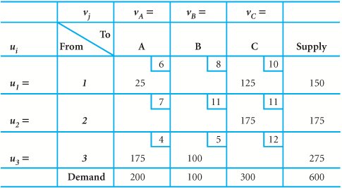
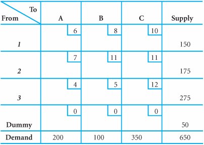
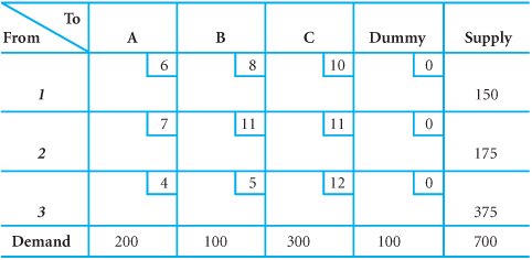
The Unbalanced Transportation ModelThus far, the methods for determining an initial solution and an optimal solution have been demonstrated within the context of a balanced transportation model. Realistically, however, an unbalanced problem is a more likely occurrence. Consider our example of transporting wheat. By changing the demand at Cincinnati to 350 tons, we create a situation in which total demand is 650 tons and total supply is 600 tons. To compensate for this difference in the transportation tableau, a "dummy" row is added to the tableau, as shown in Table B-29. The dummy row is assigned a supply of 50 tons to balance the model. The additional 50 tons demanded, which cannot be supplied, will be allocated to a cell in the dummy row. The transportation costs for the cells in the dummy row are zero because the tons allocated to these cells are not amounts really transported but the amounts by which demand was not met. These dummy cells are, in effect, slack variables . Table B-29. An Unbalanced Model (Demand > Supply) When demand exceeds supply, a dummy row is added to the tableau . Now consider our example with the supply at Des Moines increased to 375 tons. This increases total supply to 700 tons, while total demand remains at 600 tons. To compensate for this imbalance, we add a dummy column instead of a dummy row, as shown in Table B-30. Table B-30. An Unbalanced Model (Supply > Demand)(This item is displayed on page B-20 in the print version) When a supply exceeds demand, a dummy column is added to the tableau . The addition of a dummy row or a dummy column has no effect on the initial solution methods or on the methods for determining an optimal solution. The dummy row or column cells are treated the same as any other tableau cell. For example, in the minimum cell cost method, three cells would be tied for the minimum cost cell, each with a cost of zero. In this case (or any time there is a tie between cells) the tie would be broken arbitrarily. DegeneracyIn all the tableaus showing a solution to the wheat transportation problem, the following condition was met. m rows + n columns - 1 = the number of cells with allocations For example, in any of the balanced tableaus for wheat transportation, the number of rows was three (i.e., m = 3) and the number of columns was three (i.e., n = 3); thus, 3 + 3 - 1 = 5 cells with allocations. These tableaus always had five cells with allocations; thus, our condition for normal solution was met. When this condition is not met and fewer than m + n - 1 cells have allocations, the tableau is said to be degenerate . In a transportation tableau with m rows and n columns, there must be m + n - 1 cells with allocations; if not, it is degenerate . Consider the wheat transportation example with the supply values changed to the amounts shown in Table B-31. The initial solution shown in this tableau was developed using the minimum cell cost method. Table B-31. The Minimum Cell Cost Initial Solution The tableau shown in Table B-31 does not meet the condition m + n - 1 = the number of cells with allocations 3 + 3 - 1 = 5 cells because there are only four cells with allocations. The difficulty resulting from a degenerate solution is that neither the stepping-stone method nor MODI will work unless the preceding condition is met (there is an appropriate number of cells with allocations). When the tableau is degenerate, a closed path cannot be completed for all cells in the stepping-stone method, and not all the u i + v j = c ij computations can be completed in MODI. For example, a closed path cannot be determined for cell 1A in Table B-31. In a degenerate tableau, not all of the stepping-stone paths or MODI equations can be developed . To create a closed path, one of the empty cells must be artificially designated as a cell with an allocation. Cell 1A in Table B-32 is designated arbitrarily as a cell with artificial allocation of zero. (However, any symbol, such as ˜, could be used to signify the artificial allocation.) This indicates that this cell will be treated as a cell with an allocation in determining stepping-stone paths or MODI formulas, although there is no real allocation in this cell. Notice that the location of 0 was arbitrary because there is no general rule for allocating the artificial cell. Allocating zero to a cell does not guarantee that all of the steppingstone paths can be determined. Table B-32. The Initial Solution To rectify a degenerate tableau, an empty cell must artificially be treated as an occupied cell . For example, if zero had been allocated to cell 2B instead of to cell 1A, none of the stepping-stone paths could have been determined, even though technically the tableau would no longer be degenerate. In such a case, the zero must be reallocated to another cell and all paths determined again. This process must be repeated until an artificial allocation has been made that will enable the determination of all paths. In most cases, however, there is more than one possible cell to which such an allocation can be made. The stepping-stone paths and cost changes for this tableau follow. Because cell 3B shows a $1 decrease in cost for every ton of wheat allocated to it, we will allocate 100 tons to cell 3B. This results in the tableau shown in Table B-33. Table B-33. The Second Stepping-Stone Iteration(This item is displayed on page B-22 in the print version) Notice that the solution in Table B-33 now meets the condition m + n - 1 = 5. Thus, in applying the stepping-stone method (or MODI) to this tableau, it is not necessary to make an artificial allocation to an empty cell. It is quite possible to begin the solution process with a normal tableau and have it become degenerate or begin with a degenerate tableau and have it become normal. If it had been indicated that the cell with the zero should have units subtracted from it, no actual units could have been subtracted. In that case the zero would have been moved to the cell that represents the entering variable. (The solution shown in Table B-33 is optimal; however, a multiple optimal solution exists at cell 2A.) A normal problem can become degenerate at any iteration and vice versa . Prohibited RoutesSometimes one or more of the routes in the transportation model are prohibited . That is, units cannot be transported from a particular source to a particular destination. When this situation occurs, we must make sure that no units in the optimal solution are allocated to the cell representing this route. In our study of the simplex tableau, we learned that assigning a large relative cost or a coefficient of m to a variable would keep it out of the final solution. This same principle can be used in a transportation model for a prohibited route. A value of m is assigned as the transportation cost for a cell that represents a prohibited route. Thus, when the prohibited cell is evaluated, it will always contain a large positive cost change of m , which will keep it from being selected as an entering variable. A prohibited route is assigned a large cost such as m so that it will never receive an allocation . | ||||||||||||||||||||||||||||||||||||||||||||||||||||||||||||||||

 inequality because all of the tons of wheat available will be needed to meet the
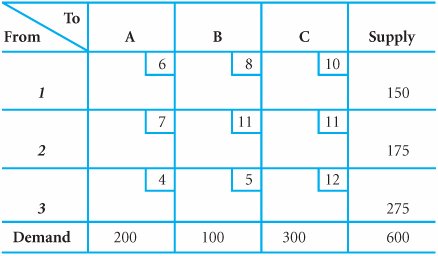


EAN: 2147483647
Pages: 358