The Basic EOQ Model | Introduction to Management Science (10th Edition)

[Page 733 ( continued )]

The simplest form of the economic order quantity model on which all other model versions are based is called the basic EOQ model. It is essentially a single formula for determining the optimal order size that minimizes the sum of carrying costs and ordering costs. The model formula is derived under a set of simplifying and restrictive assumptions, as follows :

Demand is known with certainty and is relatively constant over time.
No shortages are allowed.
Lead time for the receipt of orders is constant.
The order quantity is received all at once.

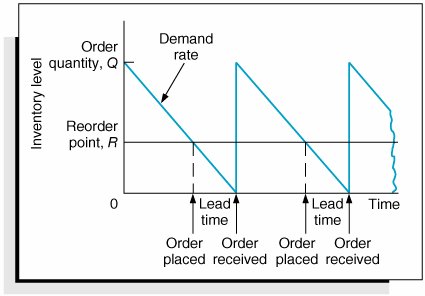
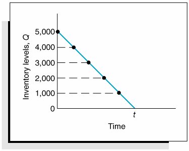
EOQ is the optimal order quantity that will minimize total inventory costs .

Assumptions of the EOQ model include constant demand, no shortages, constant lead time, and instantaneous order receipt .

The graph in Figure 16.1 reflects these basic model assumptions.

Figure 16.1. The inventory order cycle

[Page 734]

Figure 16.1 describes the continuous inventory order cycle system inherent in the EOQ model. An order quantity, Q , is received and is used up over time at a constant rate. When the inventory level decreases to the reorder point, R , a new order is placed, and a period of time, referred to as the lead time , is required for delivery. The order is received all at once, just at the moment when demand depletes the entire stock of inventory (and the inventory level reaches zero), thus allowing no shortages. This cycle is continuously repeated for the same order quantity, reorder point, and lead time.

As we mentioned earlier, Q is the order size that minimizes the sum of carrying costs and holding costs. These two costs react inversely to each other in response to an increase in the order size. As the order size increases, fewer orders are required, causing the ordering cost to decline, whereas the average amount of inventory on hand increases , resulting in an increase in carrying costs. Thus, in effect, the optimal order quantity represents a compromise between these two conflicting costs.

Carrying Cost

Carrying cost is usually expressed on a per-unit basis for some period of time (although it is sometimes given as a percentage of average inventory). Traditionally, the carrying cost is referred to on an annual basis (i.e., per year).

The total carrying cost is determined by the amount of inventory on hand during the year. The amount of inventory available during the year is illustrated in Figure 16.2.

Figure 16.2. Inventory usage

In Figure 16.2, Q represents the size of the order needed to replenish inventory, which is what a manager wants to determine. The line connecting Q to time, t , in our graph represents the rate at which inventory is depleted, or demand , during the time period, t . Demand is assumed to be known with certainty and is thus constant, which explains why the line representing demand is straight. Also, notice that inventory never goes below zero; shortages do not exist. In addition, when the inventory level does reach zero, it is assumed that an order arrives immediately after an infinitely small passage of time, a condition referred to as instantaneous receipt . This is a simplifying assumption that we will maintain for the moment.

Referring to Figure 16.2, we can see that the amount of inventory is Q , the size of the order, for an infinitely small period of time because Q is always being depleted by demand. Similarly, the amount of inventory is zero for an infinitely small period of time because the only time there is no inventory is at the specific time t . Thus, the amount of inventory available is somewhere between these two extremes. A logical deduction is that the amount of inventory available is the average inventory level, defined as

[Page 735]

To verify this relationship, we can specify any number of pointsvalues of Q over the entire time period, t , and divide by the number of points. For example, if Q = 5,000, the six points designated from 5,000 to 0, as shown in Figure 16.3, are summed and divided by 6:

Figure 16.3. Levels of Q

Alternatively, we can sum just the two extreme points (which also encompass the range of time, t ) and divide by 2. This also equals 2,500. This computation is the same, in principle, as adding Q and 0 and dividing by 2, which equals Q /2. This relationship for average inventory is maintained , regardless of the size of the order, Q , or the frequency of orders (i.e., the time period, t ). Thus, the average inventory on an annual basis is also Q /2, as shown in Figure 16.4.

Figure 16.4. Annual average inventory

[Page 736]

Now that we know that the amount of inventory available on an annual basis is the average inventory, Q /2, we can determine the total annual carrying cost by multiplying the average number of units in inventory by the carrying cost per unit per year, C _c :

Ordering Cost

The total annual ordering cost is computed by multiplying the cost per order, designated as C _o , by the number of orders per year. Because annual demand is assumed to be known and constant, the number of orders will be D / Q , where Q is the order size:

The only variable in this equation is Q ; both C _o and D are constant parameters. In other words, demand is known with certainty. Thus, the relative magnitude of the ordering cost is dependent upon the order size.

Total Inventory Cost

The total annual inventory cost is simply the sum of the ordering and carrying costs:

These cost functions are shown in Figure 16.5. Notice the inverse relationship between ordering cost and carrying cost, resulting in a convex total cost curve.

Figure 16.5. The EOQ cost model

Observe the general upward trend of the total carrying cost curve. As the order size Q (shown on the horizontal axis) increases, the total carrying cost (shown on the vertical axis) increases. This is logical because larger orders will result in more units carried in inventory. Next, observe the ordering cost curve in Figure 16.5. As the order size, Q , increases, the ordering cost decreases (just the opposite of what occurred with the carrying cost). This is logical because an increase in the size of the orders will result in fewer orders being placed each year. Because one cost increases as the other decreases, the result of summing the two costs is a convex total cost curve.

[Page 737]

The optimal order quantity occurs at the point in Figure 16.5 where the total cost curve is at a minimum, which also coincides exactly with the point where the ordering cost curve intersects with the carrying cost curve. This enables us to determine the optimal value of Q by equating the two cost functions and solving for Q , as follows:

The optimal value of Q corresponds to the lowest point on the total cost curve .

Alternatively, the optimal value of Q can be determined by differentiating the total cost curve with respect to Q , setting the resulting function equal to zero (the slope at the minimum point on the total cost curve), and solving for Q , as follows:

The total minimum cost is determined by substituting the value for the optimal order size, Q _opt , into the total cost equation:

We will use the following example to demonstrate how the optimal value of Q is computed. The I-75 Carpet Discount Store in north Georgia stocks carpet in its warehouse and sells it through an adjoining showroom. The store keeps several brands and styles of carpet in stock; however, its biggest seller is Super Shag carpet. The store wants to determine the optimal order size and total inventory cost for this brand of carpet, given an estimated annual demand of 10,000 yards of carpet, an annual carrying cost of $0.75 per yard, and an ordering cost of $150. The store would also like to know the number of orders that will be made annually and the time between orders (i.e., the order cycle), given that the store is open every day except Sunday, Thanksgiving Day, and Christmas Day (which is not on a Sunday).

We can summarize the model parameters as follows:

[Page 738]

The optimal order size is computed as follows:

The total annual inventory cost is determined by substituting Q _opt into the total cost formula, as follows:

The number of orders per year is computed as follows:

Given that the store is open 311 days annually (365 days minus 52 Sundays, plus Thanksgiving and Christmas), the order cycle is determined as follows:

It should be noted that the optimal order quantity determined in this example, and in general, is an approximate value because it is based on estimates of carrying and ordering costs as well as uncertain demand (although all these parameters are treated as known, certain values in the EOQ model). Thus, in practice it is acceptable to round off the Q values to the nearest whole number. The precision of a decimal place generally is neither necessary nor appropriate. In addition, because the optimal order quantity is computed from a square root, errors or variations in the cost parameters and demand tend to be dampened. For instance, if the order cost had actually been a third higher, or $200, the resulting optimal order size would have varied by about 15% (i.e., 2,390 yards instead of 2,000 yards). In addition, variations in both inventory costs will tend to offset each other because they have an inverse relationship. As a result, the EOQ model is relatively robust, or resilient to errors in the cost estimates and demand, which has tended to enhance its popularity.

The EOQ model is robust; because Q is a square root, errors in the estimation of D, C _c , and C _o are dampened .

EOQ Analysis Over Time

One aspect of inventory analysis that can be confusing is the time frame encompassed by the analysis. Therefore, we will digress for just a moment to discuss this aspect of EOQ analysis.

Recall that previously we developed the EOQ model "regardless of order size, Q , and time, t ." Now we will verify this condition. We will do so by developing our EOQ model on a monthly basis . First, demand is equal to 833.3 yards per month (which we determined by dividing the annual demand of 10,000 yards by 12 months). Next, by dividing the annual carrying cost, C _c , of $0.75 by 12, we get the monthly (per-unit) carrying cost: C _c = $0.0625. (The ordering cost of $150 is not related to time.) We thus have the values

[Page 739]

D = 833.3 yd. per month

C _c = $0.0625 per yd. per month

C _o = $150 per order

which we can substitute into our EOQ formula:

This is the same optimal order size that we determined on an annual basis. Now we will compute total monthly inventory cost:

To convert this monthly total cost to an annual cost, we multiply it by 12 (months):

total annual inventory cost = ($125)(12) = $1,500

This brief example demonstrates that regardless of the time period encompassed by EOQ analysis, the economic order quantity ( Q _opt ) is the same.