The EOQ Model with Noninstantaneous Receipt
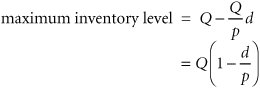
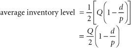
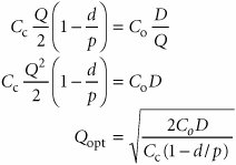
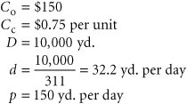
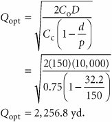
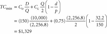
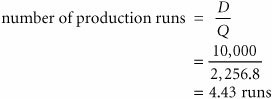
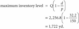
| A variation of the basic EOQ model is achieved when the assumption that orders are received all at once is relaxed . This version of the EOQ model is known as the noninstantaneous receipt model , also referred to as the gradual usage , or production lot size , model . In this EOQ variation, the order quantity is received gradually over time and the inventory level is depleted at the same time it is being replenished. This is a situation most commonly found when the inventory user is also the producer, as, for example, in a manufacturing operation where a part is produced to use in a larger assembly. This situation can also occur when orders are delivered gradually over time or the retailer and producer of a product are one and the same. The noninstantaneous receipt model is illustrated graphically in Figure 16.6, which highlights the difference between this variation and the basic EOQ model. Figure 16.6. The EOQ model with noninstantaneous order receipt(This item is displayed on page 740 in the print version)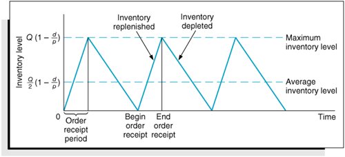 The noninstantaneous receipt model relaxes the assumption that Q is received all at once . The ordering cost component of the basic EOQ model does not change as a result of the gradual replenishment of the inventory level because it is dependent only on the number of annual orders. However, the carrying cost component is not the same for this model variation because average inventory is different. In the basic EOQ model, average inventory was half the maximum inventory level, or Q /2, but in this variation, the maximum inventory level is not simply Q ; it is an amount somewhat lower than Q , adjusted for the fact that the order quantity is depleted during the order receipt period. To determine the average inventory level, we define the following parameters that are unique to this model: p = daily rate at which the order is received over time, also known as the production rate d = the daily rate at which inventory is demanded The demand rate cannot exceed the production rate because we are still assuming that no shortages are possible, and if d = p , then there is no order size because items are used as fast as they are produced. Thus, for this model, the production rate must exceed the demand rate, or p > d . Observing Figure 16.6, the time required to receive an order is the order quantity divided by the rate at which the order is received, or Q/p . For example, if the order size is 100 units and the production rate, p , is 20 units per day, the order will be received in 5 days. The amount of inventory that will be depleted or used up during this time period is determined by multiplying by the demand rate, or (Q/p)d . For example, if it takes 5 days to receive the order and during this time inventory is depleted at the rate of 2 units per day, then a total of 10 units is used. As a result, the maximum amount of inventory that is on hand is the order size minus the amount depleted during the receipt period, computed as follows and shown earlier in Figure 16.6: Because this is the maximum inventory level, the average inventory level is determined by dividing this amount by 2, as follows: The total carrying cost, using this function for average inventory, is Thus, the total annual inventory cost is determined according to the following formula: The total inventory cost is a function of two other costs, just as in our previous EOQ model. Thus, the minimum inventory cost occurs when the total cost curve is lowest and where the carrying cost curve and ordering cost curve intersect (see Figure 16.5). Therefore, to find optimal Q opt , we equate total carrying cost with total ordering cost: For our previous example we will now assume that the I-75 Carpet Discount Store has its own manufacturing facility, in which it produces Super Shag carpet. We will further assume that the ordering cost, C o , is the cost of setting up the production process to make Super Shag carpet. Recall that C c = $0.75 per yard and D = 10,000 yards per year. The manufacturing facility operates the same days the store is open (i.e., 311 days) and produces 150 yards of the carpet per day. The optimal order size, the total inventory cost, the length of time to receive an order, the number of orders per year, and the maximum inventory level are computed as follows: The optimal order size is determined as follows: This value is substituted into the following formula to determine total minimum annual inventory cost: The length of time to receive an order for this type of manufacturing operation is commonly called the length of the production run . It is computed as follows: The number of orders per year is actually the number of production runs that will be made, computed as follows: Finally, the maximum inventory level is computed as follows: |
EAN: 2147483647
Pages: 358