Time Series Forecasting Using Excel
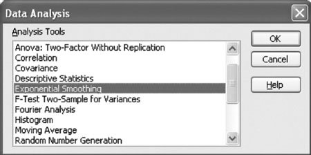
| All the time series forecasts we have presented can also be developed with Excel spreadsheets. Exhibit 15.1 shows an Excel spreadsheet set up to compute the exponentially smoothed forecast and adjusted exponentially smoothed forecast for the PM Computer Services example summarized in Table 15.5. Notice that the formula for computing the trend factor in cell D10 is shown on the formula bar on the top of the spreadsheet. The adjusted forecast in column E is computed by typing the formula = C9 +D9 in cell E9 and copying it to cells E10:E20 (using the "Copy" and "Paste" options that appear after clicking the right mouse button). Exhibit 15.1.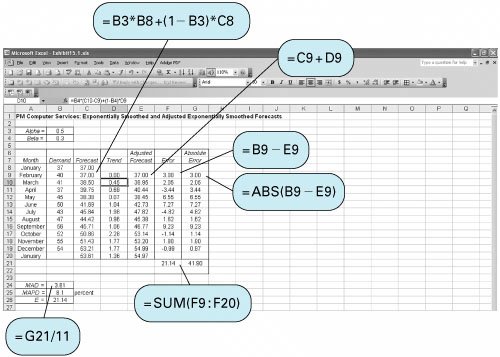 The exponential smoothing forecast can also be developed directly from Excel without "customizing" a spreadsheet and entering our own formulas, as we did in Exhibit 15.1. From the "Tools" menu at the top of the spreadsheet, select the "Data Analysis" option. (If your "Tools" menu does not include this menu item, you should add it by accessing the "Add-ins" option from the "Tools" menu or by loading from the original Excel or office software.) Exhibit 15.2 shows the Data Analysis window and the "Exponential Smoothing" menu item you should select and then click on "OK." The resulting Exponential Smoothing window is shown in Exhibit 15.3. The input range includes the demand values in column B in Exhibit 15.1, the damping factor is alpha ( a ), which in this case is 0.5, and the output should be placed in column C in Exhibit 15.1. Clicking on "OK" will result in the same forecast values in column C of Exhibit 15.1 that we computed using our own exponential smoothing formula. Note that the "Data Analysis" group of analysis tools does not have an adjusted exponential smoothing selection; that is the reason we developed our own customized spreadsheet in Exhibit 15.1. The "Data Analysis" tools also have a "Moving Average" menu item from which a moving average forecast can be computed. Exhibit 15.2. Exhibit 15.3.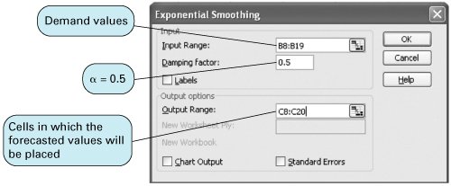 Excel can also be used to develop seasonally adjusted forecasts. Exhibit 15.4 shows an Excel spreadsheet set up to develop the seasonally adjusted forecast for the demand for turkeys at Wishbone Farms. You will notice that the seasonally adjusted forecasts for each quarter are slightly different from the forecasts computed manually (e.g., SF 1 with Excel equals 16.43, whereas SF 1 computed manually equals 16.28). This is due to the rounding done in the manual computations . Exhibit 15.4.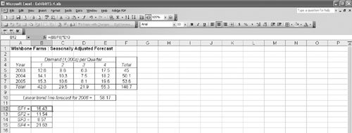 Computing the Exponential Smoothing Forecast with Excel QMIn Chapter 1 we introduced Excel QM, a set of spreadsheet macros that we have also used in several other chapters. Excel QM includes a spreadsheet macro for exponential smoothing. After it is activated, the Excel QM menu is accessed by clicking on "QM" on the menu bar at the top of the spreadsheet. Clicking on "Forecasting" from this menu results in a Spreadsheet Initialization window, in which you enter the problem title and the number of periods of past demand. Clicking on "OK" will result in the spreadsheet shown in Exhibit 15.5. Intially, this spreadsheet will have example values in the (shaded) data cells, B7 and B10:B21 . Thus, the first step in using this macro is to type in the data for our PM Computer Services problem: alpha ( a ) = 0.50 in cell B7 and our demand values in cells B10:B21 . The forecast results are computed automatically from formulas already embedded in the spreadsheet. The resulting next -period forecast for January is shown in cell B26, and the monthly forecasts are shown in cells D10:D21 . (Do not confuse this exponentially smoothed forecast and the values for MAD and the like with the adjusted exponentially smoothed forecast and MAD value in Exhibit 15.1.) Exhibit 15.5.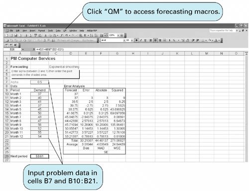 |
EAN: 2147483647
Pages: 358