The Multiple-Server Waiting Line
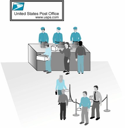
The Multiple-Server Waiting LineSlightly more complex than the single-server queuing system is the single waiting line being serviced by more than one server (i.e., multiple servers). Examples of this type of waiting line include an airline ticket and check-in counter where passengers line up in a single line, waiting for one of several agents for service, and a post office line, where customers in a single line wait for service from several postal clerks. Figure 13.3 illustrates this type of multiple-server queuing system . In multiple-server models , two or more independent servers in parallel serve a single waiting line . As an example of this type of system, consider the customer service department of the Biggs Department Store. The customer service department of the store has a waiting room in which chairs are placed along the wall, in effect forming a single waiting line. Customers come to this area with questions or complaints or to clarify matters regarding credit card bills. The customers are served by three store representatives, each located in a partitioned stall. Customers are served on a first-come, first- served basis. Figure 13.3. A multiple-server waiting line The store management wants to analyze this queuing system because excessive waiting times can make customers angry enough to shop at other stores. Typically, customers who come to this area have some problem and thus are impatient anyway. Waiting a long time serves only to increase their impatience. First, the queuing formulas for a multiple-server queuing system will be presented. These formulas, like single-server model formulas, have been developed on the assumption of a first-come, first-served queue discipline, Poisson arrivals, exponential service times , and an infinite calling population . The parameters of the multiple-server model are as follows :
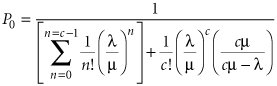
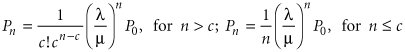
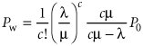
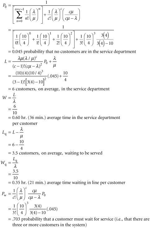
The formulas for the operating characteristics of the multiple-server model are as follows. c µ > l : the total number of servers must be able to serve customers faster than they arrive . The probability that there are no customers in the system (all servers are idle) is The probability of n customers in the queuing system is The average number of customers in the queuing system is The average time a customer spends in the queuing system (waiting and being served) is The average number of customers in the queue is The average time a customer spends in the queue, waiting to be served, is The probability that a customer arriving in the system must wait for service (i.e., the probability that all the servers are busy) is Notice in the foregoing formulas that if c = 1 (i.e., if there is one server), then these formulas become the single-server formulas presented previously in this chapter. Returning to our example, let us assume that a survey of the customer service department for a 12-month period shows that the arrival rate and service rate are as follows: l = 10 customers per hr. arrive at the service department µ = 4 customers per hr. can be served by each store representative In addition, recall that this is a three-server queuing system; therefore, c = 3 store representatives Using the multiple-server model formulas, we can compute the following operating characteristics for the service department: The department store's management has observed that customers are frustrated by the relatively long waiting time of 21 minutes and the .703 probability of waiting. To try to improve matters, management has decided to consider the addition of an extra service representative. The operating characteristics for this system must be recomputed with c = 4 service representatives. Substituting this value along with l and µ into our queuing formulas results in the following operating characteristics:
As in our previous example of the single-server system, the queuing operating characteristics provide input into the decision-making process, and the decision criteria are the waiting costs and service costs. The department store management would have to consider the cost of the extra service representative, as compared to the dramatic decrease in customer waiting time from 21 minutes to 3 minutes, in making a decision. Computer Solution of the Multiple-Server Model with Excel and Excel QMThe multiple-server model is somewhat cumbersome to set up in a spreadsheet format because of the necessity to enter some of the complex queuing formulas for this model into spreadsheet cells . Exhibit 13.11 shows a spreadsheet set up for our Biggs Department Store multiple-server example. Exhibit 13.11.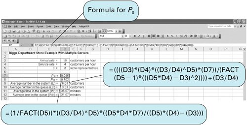 The formula for P in cell D7 is shown on the formula bar at the top of the spreadsheet. As you can see, it is long and complex. The specific summation terms in P for our example are entered directly into the formula. Thus, for a larger problem with a larger number of servers, additional summation terms would have to be entered. The term FACT() takes the factorial of a number or numbers in a cell. For example, FACT(1) is 1! Notice also that two of the other more complex formulas in this model for P w and L are shown in callout boxes attached to Exhibit 13.11. Solution of the multiple-server model, as with some of the other more complex queuing models, can be tedious using Excel spreadsheets. Excel QM is particularly useful for solving these more complex queuing models. Exhibit 13.12 shows the Excel QM spreadsheet for our Biggs Department Store example. As with other queuing models we have solved with an Excel QM queuing macro, all the formulas are already embedded in this spreadsheet; all that is required in this case is that the arrival and service rates and number of servers be entered in cells B7:B9; the operating characteristics in cells E7:E12 are computed automatically. Exhibit 13.12.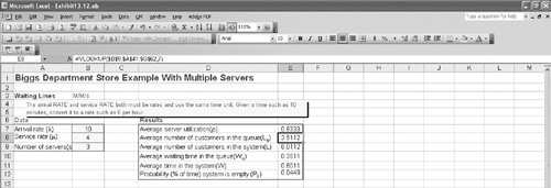 Computer Solution of the Multiple-Server Model with QM for WindowsExhibit 13.13 shows the QM for Windows solution screen for the Biggs Department Store multiple-server model example. Exhibit 13.13.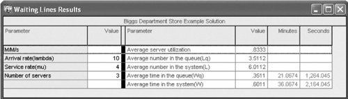 |
EAN: 2147483647
Pages: 358