Finite Calling Population
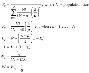
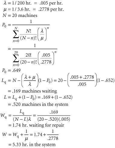
| For some waiting line systems there is a specific, limited number of potential customers that can arrive at the service facility. This is referred to as a finite calling population . As an example of this type of system, consider the Wheelco Manufacturing Company. With a finite calling population the customers from which arrivals originate are limited . Wheelco Manufacturing operates a shop that includes 20 machines. Due to the type of work performed in the shop, there is a lot of wear and tear on the machines, and they require frequent repair. When a machine breaks down, it is tagged for repair, with the date of the breakdown noted and a repair person is called. The company has one senior repair person and an assistant. They repair the machines in the same order in which they break down (a first-in, first-out queue discipline). Machines break down according to a Poisson distribution, and the service times are exponentially distributed. The finite calling population for this example is the 20 machines in the shop, which we will designate as N . The single-server model with a Poisson arrival and exponential service times and a finite calling population has the following set of formulas for determining operating characteristics. l in this model is the arrival rate for each member of the population: The formulas for P and P n are both relatively complex and can be cumbersome to compute manually. As a result, tables are often used to compute these values, given l and µ. Alternatively, the queuing module in QM for Windows has the capability to solve the finite calling population model, which we will demonstrate . Returning to our example of the Wheelco Manufacturing Company, each machine operates an average of 200 hours before breaking down and a repair person is called. The average time to repair a machine is 3.6 hours. The breakdown rate is Poisson distributed, and the service time is exponentially distributed. The company would like an analysis of machine idle time due to breakdowns to determine whether the present repair staff is sufficient. Using the formulas we developed for the single-server model with finite calling population, we can determine the operating characteristics for the machine repair system, as follows : These results show that the repair person and assistant are busy 35% of the time repairing machines. Of the 20 machines, an average of .52, or 2.6%, are broken down, waiting for repair, or under repair. Each broken-down machine is idle (broken down, waiting for repair, or under repair) an average of 5.33 hours. Thus the system seems adequate. Computer Solution of the Finite Calling Population Model with Excel and Excel QMThe finite population queuing model can be tedious to solve by using an Excel spreadsheet because of the complexity of entering the formula for P in the spreadsheet. An array must be created for the N components required by the summation in the denominator of the formula for P . Exhibit 13.8 shows the Excel spreadsheet for the Wheelco Manufacturing Company example, with this summation array in cells F4:G26 . Exhibit 13.8.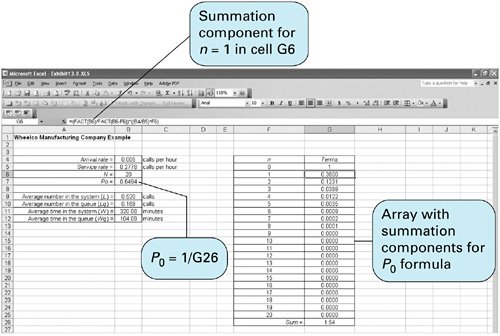 This is a model in which the spreadsheet macro in Excel QM is especially useful. The finite population model is accessed from the "QM" menu on the menu bar at the top of the spreadsheet. After selecting "Spreadsheet Initialization," the resulting spreadsheet for our Wheelco Manufacturing Company example is shown in Exhibit 13.9. As in our other Excel QM examples, the spreadsheet initially includes example data values. The first step is to enter the parameters for our own example in cells B7:B9 as shown in Exhibit 13.9. Exhibit 13.9.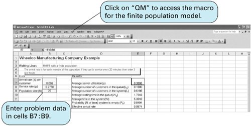 Computer Solution of the Finite Calling Population Model with QM for WindowsQM for Windows is especially useful for solving the finite calling population model because the formulas are complex and their manual solution can be tedious and time-consuming . Exhibit 13.10 includes the QM for Windows solution screen for the Wheelco Manufacturing Company example. Exhibit 13.10.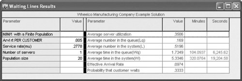 |
EAN: 2147483647
Pages: 358