The Analytical Hierarchy Process
| Goal programming is a method that provides us with a mathematical "quantity" for the decision variables that best achieves a set of goals. It answers the question "How much?" The analytical hierarchy process ( AHP ), developed by Thomas Saaty, is a method for ranking decision alternatives and selecting the best one when the decision maker has multiple objectives, or criteria, on which to base the decision. Thus, it answers the question "Which one?" A decision maker usually has several alternatives from which to choose when making a decision. For example, someone buying a house might have several houses for sale from which to choose; someone buying a new car might have several makes and styles to consider; and a prospective student might select a college to attend from a group of schools. In each of these examples, the decision maker would typically make a decision based on how the alternatives compare, according to several criteria. For example, a home buyer might consider the cost, proximity of schools , trees, neighborhood, and public transportation when comparing several houses; a car buyer might compare different cars based on price, interior comfort , mileage per gallon, and appearance. In each case, the decision maker will select the alternative that best meets his or her decision criteria. AHP is a process for developing a numeric score to rank each decision alternative, based on how well each alternative meets the decision maker's criteria. AHP is a method for ranking decision alternatives and selecting the best one given multiple criteria . We will demonstrate AHP by using an example. Southcorp Development builds and operates shopping malls around the country. The company has identified three potential sites for its latest project, near Atlanta, Birmingham, and Charlotte. The company has identified four primary criteria on which it will compare the sites(1) the customer market base (including overall market size and population at different age levels); (2) income level; (3) infrastructure (including utilities and roads ); and (4) transportation (i.e., proximity to interstate highways for supplier deliveries and customer access).
The overall objective of the company is to select the best site. This goal is at the top of the hierarchy of the problem. At the next (second) level of the hierarchy, we determine how the four criteria contribute to achieving the objective. At the level of the problem hierarchy , we determine how each of the three alternatives (Atlanta, Birmingham, and Charlotte) contributes to each of the four criteria. The general mathematical process involved in AHP is to establish preferences at each of these hierarchical levels. First, we mathematically determine our preferences for each site for each criterion. For example, we first determine our site preferences for the customer market base. We might decide that Atlanta has a better market base than the other two cities; that is, we prefer Atlanta for the customer market criterion. Then we determine our site preferences for income level, and so on. Next, we mathematically determine our preferences for the criteriathat is, which of the four criteria is most important, which is the next most important, and so on. For example, we might decide that the customer market is a more important criterion than the others. Finally, we combine these two sets of preferencesfor sites within each criterion and for the four criteriato mathematically derive a score for each site, with the highest score being the best. In the following sections we describe these general steps in greater detail. Pairwise ComparisonsIn AHP the decision maker determines how well each alternative "scores" on a criterion by using pairwise comparisons . In a pairwise comparison, the decision maker compares two alternatives (i.e., a pair) according to one criterion and indicates a preference. For example, Southcorp might compare the Atlanta (A) site with the Birmingham (B) site and decide which one it prefers according to the customer market criterion. These comparisons are made by using a preference scale , which assigns numeric values to different levels of preference. In a pairwise comparison, two alternatives are compared according to a criterion, and one is preferred . A preference scale assigns numeric values to different levels of preference . The standard preference scale used for AHP is shown in Table 9.1. This scale has been determined by experienced researchers in AHP to be a reasonable basis for comparing two items or alternatives. Each rating on the scale is based on a comparison of two items. For example, if the Atlanta site is "moderately preferred" to the Birmingham site, then a value of 3 is assigned to this particular comparison. The rating of 3 is a measure of the decision maker's preference for one of the alternatives over the other. Table 9.1. Preference scale for pairwise comparisons
If Southcorp compares Atlanta to Birmingham and moderately prefers Atlanta, resulting in a comparison value of 3 for the customer market criterion, it is not necessary for Southcorp to compare Birmingham to Atlanta to determine a separate preference value for this " opposite " comparison. The preference value of B for A is simply the reciprocal or inverse of the preference of A for B. Thus, in our example if the preference value of Atlanta for Birmingham is 3, the preference value of Birmingham for Atlanta is 1/3. Southcorp's pairwise comparison ratings for each of the three sites for the customer market criterion are summarized in a matrix, a rectangular array of numbers . This pairwise comparison matrix will have a number of rows and columns equal to the decision alternatives:
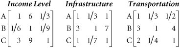
A pairwise comparison matrix summarizes the pairwise comparisons for a criterion . This matrix shows that the customer market in Atlanta (A) is equally to moderately preferred (2) over the Charlotte (C) customer market, but Charlotte (C) is strongly preferred (5) over Birmingham (B). Notice that any site compared against itself, such as A compared to A, must be "equally preferred," with a preference value of 1. Thus, the values along the diagonal of our matrix must be 1s. The remaining pairwise comparison matrices for the other three criteriaincome level, infrastructure, and transportationhave been developed by Southcorp as follows : Developing Preferences Within CriteriaThe next step in AHP is to prioritize the decision alternatives within each criterion. For our site selection example, this means that we want to determine which site is the most preferred, the second most preferred, and the third most preferred for each of the four criteria. This step in AHP is referred to as synthesization . The mathematical procedure for synthesization is very complex and beyond the scope of this text. Instead, we will use an approximation method for synthesization that provides a reasonably good estimate of preference scores for each decision in each criterion. In synthesization, decision alternatives are prioritized within each criterion . The first step in developing preference scores is to sum the values in each column of the pairwise comparison matrices. The column sums for our customer market matrix are shown as follows:
Next, we divide each value in a column by its corresponding column sum. This results in a normalized matrix, as follows:
Notice that the values in each column sum to 1. The next step is to average the values in each row . At this point, we convert the fractional values in the matrix to decimals, as shown in Table 9.2. The row average for each site is also shown in Table 9.2. Table 9.2. The normalized matrix with row averages
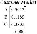
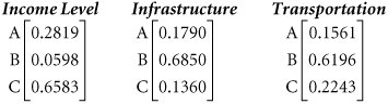
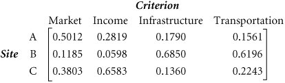
The row averages in Table 9.2 provide us with Southcorp's preferences for the three sites for the customer market criterion. The most preferred site is Atlanta, followed by Charlotte; the least preferred site (for this criterion) is Birmingham. We can write these preferences as a matrix with one column, which we will refer to as a vector : The preference vectors for the other decision criteria are computed similarly: These four preference vectors for the four criteria are summarized in a single preference matrix, shown in Table 9.3. Table 9.3. Criteria preference matrix
Ranking the CriteriaThe next step in AHP is to determine the relative importance, or weight, of the criteriathat is, to rank the criteria from most important to least important. This is accomplished the same way we ranked the sites within each criterion: using pairwise comparisons. The following pairwise comparison matrix for the four criteria in our example was developed by using the preference scale in Table 9.1:
The normalized matrix converted to decimals, with the row averages for each criterion, is shown in Table 9.4. Table 9.4. Normalized matrix for criteria, with row averages
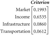
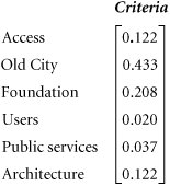
The preference vector, computed from the normalized matrix by computing the row averages in Table 9.4, is as follows: Clearly, income level is the highest-priority criterion, and customer market is second. Infrastructure and transportation appear to be relatively unimportant third- and fourth-ranked priorities in terms of the overall objective of determining the best site for the new shopping mall. The next step in AHP is to combine the preference matrices we developed for the sites for each criterion in Table 9.3 with the preceding preference vector for the four criteria. Developing an Overall RankingRecall that earlier we summarized Southcorp's preferences for each site for each criterion in a preference matrix shown in Table 9.3 and repeated as follows: In the previous section we used pairwise comparisons to develop a preference vector for the four criteria in our example: An overall score for each site is computed by multiplying the values in the criteria preference vector by the preceding criteria matrix and summing the products, as follows: site A score = 0.1993(0.5012) + 0.6535(0.2819) + 0.0860(0.1790) + 0.0612(0.1561) = 0.3091 site B score = 0.1993(0.1185) + 0.6535(0.0598) + 0.0860(0.6850) + 0.0612(0.6196) = 0.1595 site C score = 0.1993(0.3803) + 0.6535(0.6583) + 0.0860(0.1360) + 0.0612(0.2243) = 0.5314 The three sites, in order of the magnitude of their scores, result in the following AHP ranking:
Based on these scores developed by AHP, Charlotte should be selected as the site for the new shopping mall, with Atlanta ranked second and Birmingham third. To rely on this result to make its site selection decision, Southcorp must have confidence in the judgments it made in the pairwise comparisons, and it must also have confidence in AHP. However, whether the AHP-recommended decision is the one made by Southcorp or not, following this process can help identify and prioritize criteria and enlighten the company about how it makes decisions. Following is a summary of the mathematical steps used to arrive at the AHP-recommended decision:
AHP ConsistencyAHP is based primarily on the pairwise comparisons a decision maker uses to establish preferences between decision alternatives for different criteria. The normal procedure in AHP for developing these pairwise comparisons is for an interviewer to elicit verbal preferences from the decision maker, using the preference scale in Table 9.1. However, when a decision maker has to make a lot of comparisons (i.e., three or more), he or she can lose track of previous responses. Because AHP is based on these responses, it is important that they be in some sense valid and especially that the responses be consistent. That is, a preference indicated for one set of pairwise comparisons needs to be consistent with another set of comparisons.
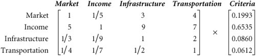
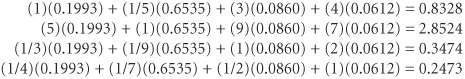
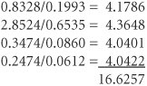
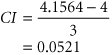
Using our site selection example, suppose for the income level criterion, Southcorp indicates that A is "very strongly preferred" to B and that A is "moderately preferred" to C. That's fine, but then suppose Southcorp says that C is "equally preferred" to B for the same criterion. That comparison is not entirely consistent with the previous two pairwise comparisons. To say that A is strongly preferred over B and moderately preferred over C and then turn around and say C is equally preferred to B does not reflect a consistent preference rating for the three sets of pairwise comparisons. A more logical comparison would be that C is preferred to B to some degree. This kind of inconsistency can creep into AHP when the decision maker is asked to make verbal responses for a lot of pairwise comparisons. In general, they are usually not a serious problem; some degree of slight inconsistency is expected. However, a consistency index can be computed that measures the degree of inconsistency in the pairwise comparisons. A consistency index measures the degree of inconsistency in pairwise comparisons . To demonstrate how to compute the consistency index ( CI ), we will check the consistency of the pairwise comparisons for the four site selection criteria. This matrix, shown as follows, is multiplied by the preference vector for the criteria: The product of the multiplication of this matrix and vector is computed as follows: Next, we divide each of these values by the corresponding weights from the criteria preference vector: If the decision maker, Southcorp, were a perfectly consistent decision maker, then each of these ratios would be exactly 4, the number of items we are comparingin this case, four criteria. Next, we average these values by summing them and dividing by 4: The consistency index, CI , is computed using the following formula: where n = the number of items being compared 4.1564 = the average we computed previously If CI = 0, then Southcorp would be a perfectly consistent decision maker. Because Southcorp is not perfectly consistent, the next question is the degree of inconsistency that is acceptable. An acceptable level of consistency is determined by comparing the CI to a random index, RI , which is the consistency index of a randomly generated pairwise comparison matrix. The RI has the values shown in Table 9.5, depending on the number of items, n , being compared. In our example, n = 4 because we are comparing four criteria. Table 9.5. RI values for n items being compared
The degree of consistency for the pairwise comparisons in the decision criteria matrix is determined by computing the ratio of CI to RI : In general, the degree of consistency is satisfactory if CI / RI < 0.10, and in this case, it is. If CI / RI > 0.10, then there are probably serious inconsistencies, and the AHP results may not be meaningful. Remember that in this instance, we have evaluated the degree of consistency only for the pairwise comparisons in the decision criteria preference matrix. This does not mean that we have verified the consistency for the entire AHP. We would still have to evaluate the pairwise comparisons for each of the four individual criterion matrices before we could be sure the entire AHP for this problem was consistent. AHP with Excel SpreadsheetsThe various computational steps involved in AHP can be accomplished with Excel spreadsheets. Exhibit 9.12 shows a spreadsheet formatted for our Southcorp site selection example. The spreadsheet includes the pairwise comparison matrix for our customer market criterion. Notice that the pairwise comparisons have been entered as fractions. We can enter fractions in Excel by dragging the cursor over the object cells , in this case B5:D7 , and then clicking on "Format" at the top of the screen. When the "Format" menu comes down, we click on "Cells" and then select "Fraction" from the menu. Exhibit 9.12.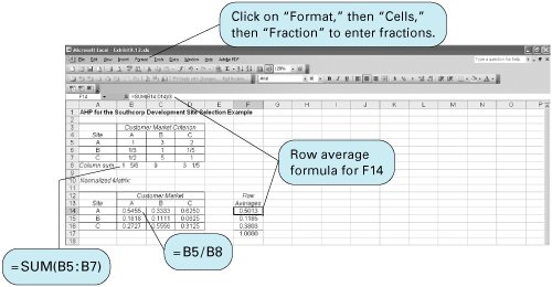 The sum for column A in the pairwise comparison matrix is obtained by inserting the formula = SUM(B5:B7) in cell B8. The sums for columns B and C can then be obtained by putting the cursor on cell B8, clicking on the right mouse button, and clicking on "Copy." Then we drag the cursor over cells B8:D8 and press the "Enter" key. This will compute the sum for the other two columns.
The cell values for the normalized matrix at the bottom of the spreadsheet in Exhibit 9.12 can be computed as follows. First, make sure you convert the cell values to decimal numbers. To start, divide the value in cell B5 by the column sum in cell B8 by typing = B5/B8 in cell B14. This results in the value 0.5455 in cell B14. Next, with the cursor on B14, click the right mouse button and then click on "Copy." Drag the cursor across cells B14:D14 and press the "Enter" key. This will compute the values for cells C14 and D14. Repeat this process for each row to complete the normalized matrix. To compute the row averages from the normalized matrix, first type the formula = SUM(B14:D14)/3 in cell F14. This formula is displayed on the formula bar at the top of the spreadsheet. This will compute the value 0.5013 in cell F14. Next, with the cursor on cell F14, click the right mouse button and copy the formula in cell F14 to F15 and F16 by dragging the cursor across cells F14:F16 . Recall that these row averages represent the preference vector for the customer market criterion. To complete this stage in AHP, we would need to compute the preference vectors for the other three criteria for income level, infrastructure, and transportation. The next step in AHP is to develop the pairwise comparison matrix and normalized matrix for our four criteria. The spreadsheet to accomplish this step is shown in Exhibit 9.13. These two matrices are constructed in the same way as the two similar matrices in Exhibit 9.12. Exhibit 9.13.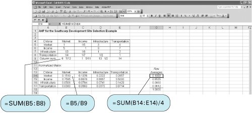 The final step in AHP is to develop an overall ranking. This requires Southcorp's preference matrix for each site for all four criteria (Table 9.3) and the preference vector for the criteria, both of which are included in the spreadsheet shown in Exhibit 9.14. Exhibit 9.14.(This item is displayed on page 416 in the print version)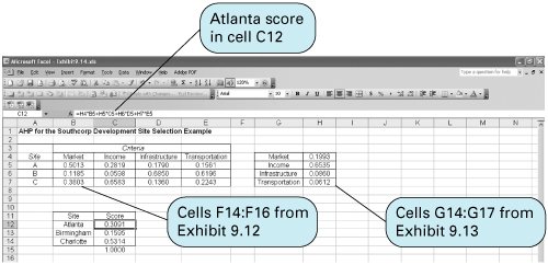 All the values in the two matrices in Exhibit 9.14 were entered as input from previous AHP steps. The score for Atlanta was computed using the formula embedded in cell C12 and shown on the formula bar. Similar formulas were used for the other two site scores in cells C13 and C14. Exhibit 9.15 shows the spreadsheet for evaluating the degree of consistency for the pairwise comparisons in the preference matrix for the four criteria. The spreadsheet is broken down into steps that are self-explanatory. Exhibit 9.15.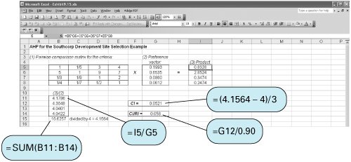 | |||||||||||||||||||||||||||||||||||||||||||||||||||||||||||||||||||||||||||||||||||||||||||||||||||||||||||||||||||||||||||||||||||||||||||||||||||||||||||||||||||||||||||||||||||||||||||||||||||||||||||||||||||||||||||||||||||||||||||||||||||||||||||||||||||


EAN: 2147483647
Pages: 358