[Page 378 (continued)]4.2. Swapping With a batch system, organizing memory into fixed partitions is simple and effective. Each job is loaded into a partition when it gets to the head of the queue. It stays in memory until it has finished. As long as enough jobs can be kept in memory to keep the CPU busy all the time, there is no reason to use anything more complicated. With timesharing systems or graphics-oriented personal computers, the situation is different. Sometimes there is not enough main memory to hold all the currently active processes, so excess processes must be kept on disk and brought in to run dynamically. Two general approaches to memory management can be used, depending (in part) on the available hardware. The simplest strategy, called swapping, consists of bringing in each process in its entirety, running it for a while, then putting it back on the disk. The other strategy, called virtual memory, allows programs to run even when they are only partially in main memory. Below we will study swapping; in Sec. 4.3 we will examine virtual memory. The operation of a swapping system is illustrated in Fig. 4-3. Initially, only process A is in memory. Then processes B and C are created or swapped in from disk. In Fig. 4-3(d) A is swapped out to disk. Then D comes in and B goes out. Finally A comes in again. Since A is now at a different location, addresses contained in it must be relocated, either by software when it is swapped in or (more likely) by hardware during program execution. Figure 4-3. Memory allocation changes as processes come into memory and leave it. The shaded regions are unused memory. (This item is displayed on page 379 in the print version) 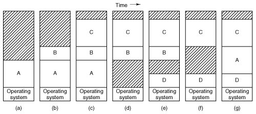
The main difference between the fixed partitions of Fig. 4-2 and the variable partitions of Fig. 4-3 is that the number, location, and size of the partitions vary dynamically in the latter as processes come and go, whereas they are fixed in the former. The flexibility of not being tied to a fixed number of partitions that may be too large or too small improves memory utilization, but it also complicates allocating and deallocating memory, as well as keeping track of it. When swapping creates multiple holes in memory, it is possible to combine them all into one big one by moving all the processes downward as far as possible. This technique is known as memory compaction. It is usually not done because it requires a lot of CPU time. For example, on a 1-GB machine that can copy at a rate of 2 GB/sec (0.5 nsec/byte) it takes about 0.5 sec to compact all of memory. That may not seem like much time, but it would be noticeably disruptive to a user watching a video stream.
[Page 379] A point that is worth making concerns how much memory should be allocated for a process when it is created or swapped in. If processes are created with a fixed size that never changes, then the allocation is simple: the operating system allocates exactly what is needed, no more and no less. If, however, processes' data segments can grow, for example, by dynamically allocating memory from a heap, as in many programming languages, a problem occurs whenever a process tries to grow. If a hole is adjacent to the process, it can be allocated and the process can be allowed to grow into the hole. On the other hand, if the process is adjacent to another process, the growing process will either have to be moved to a hole in memory large enough for it, or one or more processes will have to be swapped out to create a large enough hole. If a process cannot grow in memory and the swap area on the disk is full, the process will have to wait or be killed. If it is expected that most processes will grow as they run, it is probably a good idea to allocate a little extra memory whenever a process is swapped in or moved, to reduce the overhead associated with moving or swapping processes that no longer fit in their allocated memory. However, when swapping processes to disk, only the memory actually in use should be swapped; it is wasteful to swap the extra memory as well. In Fig. 4-4(a) we see a memory configuration in which space for growth has been allocated to two processes. Figure 4-4. (a) Allocating space for a growing data segment. (b) Allocating space for a growing stack and a growing data segment. (This item is displayed on page 380 in the print version) 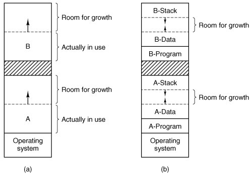
If processes can have two growing segments, for example, the data segment being used as a heap for variables that are dynamically allocated and released and a stack segment for the normal local variables and return addresses, an alternative arrangement suggests itself, namely that of Fig. 4-4(b). In this figure we see that each process illustrated has a stack at the top of its allocated memory that is growing downward, and a data segment just beyond the program text that is growing upward. The memory between them can be used for either segment. If it runs out, either the process will have to be moved to a hole with sufficient space, swapped out of memory until a large enough hole can be created, or killed.
[Page 380] 4.2.1. Memory Management with Bitmaps When memory is assigned dynamically, the operating system must manage it. In general terms, there are two ways to keep track of memory usage: bitmaps and free lists. In this section and the next one we will look at these two methods in turn. With a bitmap, memory is divided up into allocation units, perhaps as small as a few words and perhaps as large as several kilobytes. Corresponding to each allocation unit is a bit in the bitmap, which is 0 if the unit is free and 1 if it is occupied (or vice versa). Figure 4-5 shows part of memory and the corresponding bitmap. Figure 4-5. (a) A part of memory with five processes and three holes. The tick marks show the memory allocation units. The shaded regions (0 in the bitmap) are free. (b) The corresponding bitmap. (c) The same information as a list. (This item is displayed on page 381 in the print version) 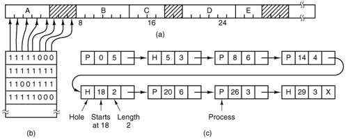
The size of the allocation unit is an important design issue. The smaller the allocation unit, the larger the bitmap. However, even with an allocation unit as small as 4 bytes, 32 bits of memory will require only 1 bit of the map. A memory of 32n bits will use n map bits, so the bitmap will take up only 1/33 of memory. If the allocation unit is chosen large, the bitmap will be smaller, but appreciable memory may be wasted in the last unit of the process if the process size is not an exact multiple of the allocation unit.
[Page 381] A bitmap provides a simple way to keep track of memory words in a fixed amount of memory because the size of the bitmap depends only on the size of memory and the size of the allocation unit. The main problem with it is that when it has been decided to bring a k unit process into memory, the memory manager must search the bitmap to find a run of k consecutive 0 bits in the map. Searching a bitmap for a run of a given length is a slow operation (because the run may straddle word boundaries in the map); this is an argument against bitmaps. 4.2.2. Memory Management with Linked Lists Another way of keeping track of memory is to maintain a linked list of allocated and free memory segments, where a segment is either a process or a hole between two processes. The memory of Fig. 4-5(a) is represented in Fig. 4-5(c) as a linked list of segments. Each entry in the list specifies a hole (H) or process (P), the address at which it starts, the length, and a pointer to the next entry. In this example, the segment list is kept sorted by address. Sorting this way has the advantage that when a process terminates or is swapped out, updating the list is straightforward. A terminating process normally has two neighbors (except when it is at the very top or very bottom of memory). These may be either processes or holes, leading to the four combinations shown in Fig. 4-6. In Fig. 4-6(a) updating the list requires replacing a P by an H. In Fig. 4-6(b) and also in Fig. 4-6(c), two entries are coalesced into one, and the list becomes one entry shorter. In Fig. 4-6(d), three entries are merged and two items are removed from the list. Since the process table slot for the terminating process will normally point to the list entry for the process itself, it may be more convenient to have the list as a double-linked list, rather than the single-linked list of Fig. 4-5(c). This structure makes it easier to find the previous entry and to see if a merge is possible.
[Page 382] Figure 4-6. Four neighbor combinations for the terminating process, X. 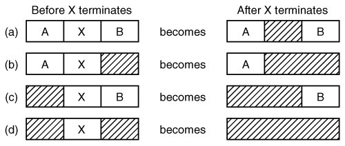
When the processes and holes are kept on a list sorted by address, several algorithms can be used to allocate memory for a newly created process (or an existing process being swapped in from disk). We assume that the memory manager knows how much memory to allocate. The simplest algorithm is first fit. The process manager scans along the list of segments until it finds a hole that is big enough. The hole is then broken up into two pieces, one for the process and one for the unused memory, except in the statistically unlikely case of an exact fit. First fit is a fast algorithm because it searches as little as possible. A minor variation of first fit is next fit. It works the same way as first fit, except that it keeps track of where it is whenever it finds a suitable hole. The next time it is called to find a hole, it starts searching the list from the place where it left off last time, instead of always at the beginning, as first fit does. Simulations by Bays (1977) show that next fit gives slightly worse performance than first fit. Another well-known algorithm is best fit. Best fit searches the entire list and takes the smallest hole that is adequate. Rather than breaking up a big hole that might be needed later, best fit tries to find a hole that is close to the actual size needed. As an example of first fit and best fit, consider Fig. 4-5 again. If a block of size 2 is needed, first fit will allocate the hole at 5, but best fit will allocate the hole at 18. Best fit is slower than first fit because it must search the entire list every time it is called. Somewhat surprisingly, it also results in more wasted memory than first fit or next fit because it tends to fill up memory with tiny, useless holes. First fit generates larger holes on the average. To get around the problem of breaking up nearly exact matches into a process and a tiny hole, one could think about worst fit, that is, always take the largest available hole, so that the hole broken off will be big enough to be useful. Simulation has shown that worst fit is not a very good idea either.
[Page 383] All four algorithms can be speeded up by maintaining separate lists for processes and holes. In this way, all of them devote their full energy to inspecting holes, not processes. The inevitable price that is paid for this speedup on allocation is the additional complexity and slowdown when deallocating memory, since a freed segment has to be removed from the process list and inserted into the hole list. If distinct lists are maintained for processes and holes, the hole list may be kept sorted on size, to make best fit faster. When best fit searches a list of holes from smallest to largest, as soon as it finds a hole that fits, it knows that the hole is the smallest one that will do the job, hence the best fit. No further searching is needed, as it is with the single list scheme. With a hole list sorted by size, first fit and best fit are equally fast, and next fit is pointless. When the holes are kept on separate lists from the processes, a small optimization is possible. Instead of having a separate set of data structures for maintaining the hole list, as is done in Fig. 4-5(c), the holes themselves can be used. The first word of each hole could be the hole size, and the second word a pointer to the following entry. The nodes of the list of Fig. 4-5(c), which require three words and one bit (P/H), are no longer needed. Yet another allocation algorithm is quick fit, which maintains separate lists for some of the more common sizes requested. For example, it might have a table with n entries, in which the first entry is a pointer to the head of a list of 4-KB holes, the second entry is a pointer to a list of 8-KB holes, the third entry a pointer to 12-KB holes, and so on. Holes of say, 21 KB, could either be put on the 20-KB list or on a special list of odd-sized holes. With quick fit, finding a hole of the required size is extremely fast, but it has the same disadvantage as all schemes that sort by hole size, namely, when a process terminates or is swapped out, finding its neighbors to see if a merge is possible is expensive. If merging is not done, memory will quickly fragment into a large number of small holes into which no processes fit. |