Category list

2.2 Equilibrium risk-free rate of interest

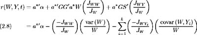
We need to determine the equilibrium values of a , r and ² . The solution to an individual's planning problem consists of an optimal physical investment policy a *, optimal consumption plan C * and the associated indirect utility function J *. By writing the portfolio allocation (physical investment) part as a quadratic programming problem, CIR [ 17 ] determine the equilibrium interest rate to be of the form:

2.3 Equilibrium expected return on any contingent claim

Considering optimal physical investment a *, and substituting the equilibrium interest rate (2.8) into (2.7e) we get the equilibrium expected return on any contingent claim:

Now, applying Ito's lemma to F ( W, Y, t ), and making use of (2.5) and (2.2):

with:

Now comparing the volatility components of (2.10) and (2.3) we have:

Substitution into (2.9) gives:

which by (2.8) becomes:

So the equilibrium expected return on any contingent claim may be written as the risk-free return rF , plus a linear combination of the first derivatives of the contingent claim price with respect to wealth W , and the state variables Y . The coefficients of these derivatives are independent of the contractual specification for that claim; hence they are the same for all contingent claims. CIR [ 17 ] explain that these coefficients may be interpreted as factor risk premia ^[4] .

^[4] Specifically from (2.11), the risk premium for the i ^th state variable Y _i is

2.4 Value of any contingent claim in equilibrium

Now comparing the drift coefficients in (2.10) and (2.3) we have:

Making use of (2.11) yields:

Rearranging terms we have a partial differential equation for the price of any contingent claim ^[5] :

This valuation equation holds for any contingent claim. Specific terminal and boundary conditions as well as the structure of , the payout flow, define the unique characteristics of a claim.

^[5] First group the coefficients of F _W and make use of (2.8) to give:

2.5 A more specialised economy

For the problem of modelling the interest rate term structure, CIR specialise the economy. They restrict the class of utility functions to those having constant relative risk aversion ^[6] . Specifically, the utility function is required to be logarithmic and independent of the state variable Y , hence:

where is a constant discount factor.

CIR [ 18 ] show that for this specialised case the indirect utility function takes the form:

for some functions h ( t ) and g ( Y,t ). By the results of the earlier Lemma

Hence we have:

Substituting into (2.8), the form of the equilibrium interest rate reduces to:

Similarly, by (2.11), the return on any contingent claim simplifies to:

For the purposes of developing a model of the interest rate term structure, CIR assume that the contractual terms of all securities are free of explicit dependence on wealth. This implies that the partial derivatives, with respect to wealth, of all securities, equal zero (i.e. F _W = F _WW = F _WY = 0). As shown above the risk-free rate and factor risk premia ^[7] are also independent of wealth. Due to this additional restriction the valuation equation for contingent claims (2.12) reduces to: 1

^[6] That is neither the interest rate, nor the security risk premia depend on the level of investor wealth.

^[7] In (2.15) the factor risk premia, that is the coefficients of F _{Y
_i} , reduce to a * ² GS ² .

Flylib.com

Category list

Similar pages

2.2 Equilibrium risk-free rate of interest