Project 6.1: Creating a New Primitive

Project Overview

By default, Maya includes relatively few primitive objects. Those it does include, with the exception of the sphere, are actually quite easily built by hand. One of the more useful primitive types Maya does not include is the Regular Polyhedron . A regular polyhedron, also called a Platonic Solid , is defined as a solid object where each face has an equal number of vertices, and all the angles of the face are equal. In addition, two spheres are defined as a Platonic Solid. The first, called the circumscribed sphere , is defined by the vertices, and the second, the inscribed sphere , is defined by the center of each face.

With all those rules, it should come as no surprise that there are five, and only five, of these objects: the tetrahedron, the cube, the octahedron, the dodecahedron, and the icosahedron. Of these, obviously artists are most familiar with the cube. However, to anyone who has played games involving dice of more or less than six sides is most familiar with the other types as well.

For our first project, we will create a script to construct an icosahedron. Icosahedrons are incredibly useful for modeling objects for video games and for use in soft body simulations involving springs, due to their inherent structural integrity. The icosahedron is also the foundation for the geodesic sphere .

This project will present the simplest way of constructing the icosahedron, without the complications of having to pass the script data or work too extensively with sub-object components . In the final project of this chapter, we will revisit the icosahedron, using what we learn in Project 6.2 to enhance the usefulness of our script.

The one disadvantage to constructing primitives with MEL rather than the API is the lack of construction history. There are ways to add some similar, albeit limited functionality to primitives created in MEL, through expressions and dynamic attributes, but for this project, simplicity is key.

Definition and Design

Our tool is rather simple; our only goal is to create a polygonal icosahedron. The shape itself is not complicated, simply made up of 20 triangular faces. Logically, the simplest way to create the icosahedron is to create each of the 20 faces and merge them together to create a single object. The important question is how to determine the co-ordinates of our icosahedron s vertices.

With this simple definition, we are able to create our flowchart, seen in Flowchart 6.1.

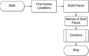
Flowchart 6.1: Icosahedron generator flowchart.

This is our first project, so the obvious simplicity is to our advantage. Looking at our diagram, we can see the need for the ability to do, at minimum, three functions with MEL.

We need to:

• Determine the vertex co-ordinates

• Create raw polygonal faces at those co-ordinates

• Merge that geometry together

Now that we have our script essentially designed and some potential problems defined, we can move on to finding solutions to those problems, which we do through research.

Research and Development

Our most pressing problem in the creation of our icosahedron is finding an equation to determine the vertex co-ordinates. Our first stop is the Internet. We can easily find definitions of the relationship between the radius of an icosahedron and the length of an edge. We could use trigonometry to build our icosahedron, since we now know the ratio of each side to each other. While this is a workable solution, a more elegant solution exists, found in the FAQ for comp.graphics.algorithms, an Internet newsgroup.

Looking at Figure 6.1, we see that the 12 vertices of an icosahedron are defined by three intersecting rectangles.

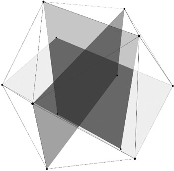
Figure 6.1: The intersecting rectangles defining the icosahedron.

These rectangles are defined by the Golden Ratio . This ratio is considered to be the ideal ration of width to height of any rectangle. How it interacts with our icosahedron stems from the fact that the Golden Ratio is a number relating to the interaction of a triangle and a circle. This means that we can use the Golden Ratio to define our vertex locations. The equation for the Golden Ratio is shown in Equation 6.1.

From this, we can derive our 12 vertex locations, where x is the Golden Ratio:

• (+/ “ 1, 0, +/ “ x )

• (0, +/ “ x , +/ “ 1)

• (+/ “ x , +/ “ 1, 0)

Implementation

Now, we will start building our script to test our vertex locations. Open a new script file, and save it within your scripts directory as  buildPolyIcosohedron.mel .

We begin by declaring our procedure, named the same as our file. Be sure to add the curly brackets to create an empty procedure, as seen in Example 6.1. Then, save your file.

Example 6.1: Declaration of our procedure.

 global proc buildPolyIcosohedron ()     {     } 

Open Maya, and create a new shelf called MEL_Companion. Using the Script Editor, create a shelf button to source and execute our script. We do this so we can update our script file and have these updates reflected when we execute the script. The code needed to do this is seen in Example 6.2.

Example 6.2: Creating a shelf button to both source and execute a script eases script development.

 source buildPolyIcosohedron ;     buildPolyIcosohedron ; 

We build this into a button simply to save us the effort of retyping the commands over and over, and freeing up the Script Editor should we want to test a section of code. If we now execute the sourcing code, nothing should happen. That s actually a good thing. Our procedure is empty, so it s not doing anything, but if Maya was unable to find the script file, and therefore the procedure, it will report an error. If this is the case, either move the script file to a location within your script path, or modify the path to the script file location.

Now that we have a fully functioning script file we can begin adding actual functionality. First up for our testing, we will want to define a variable to our Golden Ratio, as well as our vertex co-ordinates, which we will declare as vectors. We use the MEL command sqrt in the equation for the Golden Mean, but since we only execute the equation once, we do not waste excessive cycles using a divide rather than multiplying by 0.5, and we keep the equation in a familiar form, as seen in Example 6.3.

Example 6.3: Creating variables to hold the vertex positions .

 global proc buildPolyIcosohedron ()     {  // declaration and assignment of golden ratio  float $goldenMean = ((sqrt(5)-1)/2) ;  // declaration and assignment of vertices  vector $vert_01 = << 1, 0, $goldenMean >>;     vector $vert_02 = << -1, 0, $goldenMean >>;     vector $vert_03 = << 1, 0, ((-1.0) * $goldenMean) >>;     vector $vert_04 = << -1, 0, ((-1.0) * $goldenMean) >>;     vector $vert_05 = << 0, $goldenMean, 1 >>;     vector $vert_06 = << 0, $goldenMean, -1 >>;     vector $vert_07 = << 0, ((-1.0) * $goldenMean), 1  >>;     vector $vert_08 = << 0, ((-1.0) * $goldenMean), -1  >>;     vector $vert_09 = << $goldenMean, 1, 0  >>;     vector $vert_10 = << $goldenMean, -1, 0  >>;     vector $vert_11 = << ((-1.0) * $goldenMean) , 1, 0 >>;     vector $vert_12 = << ((-1.0) * $goldenMean) , -1, 0 >>;     } 

On the CD  

The text for this script is found on the companion CD-ROM as /project_01/v01/buildPolyIcosohedron.mel.

In order to check the placement of our vertices, we will now place a locator at each of our 12 co-ordinates. To discover the MEL command used to create a locator, we look in the Script Editor s history after executing the Create > Locator command from the menu and see spaceLocator “p 0 0 0 ; . Looking up the documentation for the spaceLocator command, we see that the -p is the short flag for -position , which will allow us to place each locator at our co-ordinates. If we now add the code in Example 6.4 to our script, after the variable assignment, we will add 12 locators to our scene at each of the co-ordinates defined by our variables.

Example 6.4: Creation of the locators.

  // creation of locators at each of the twelve locations  spaceLocator         -position ($vert_01.x) ($vert_01.y) ($vert_01.z)         -name "Vertex_01"         ;     spaceLocator         -position ($vert_02.x) ($vert_02.y) ($vert_02.z)          -name "Vertex_02"         ;     spaceLocator         -position ($vert_03.x) ($vert_03.y) ($vert_03.z)          -name "Vertex_03"         ;     spaceLocator         -position ($vert_04.x) ($vert_04.y) ($vert_04.z)          -name "Vertex_04"         ;     spaceLocator         -position ($vert_05.x) ($vert_05.y) ($vert_05.z)          -name "Vertex_05"         ;     spaceLocator         -position ($vert_06.x) ($vert_06.y) ($vert_06.z)          -name "Vertex_06"         ;     spaceLocator         -position ($vert_07.x) ($vert_07.y) ($vert_07.z)          -name "Vertex_07"         ;     spaceLocator         -position ($vert_08.x) ($vert_08.y) ($vert_08.z)          -name "Vertex_08"         ;     spaceLocator         -position ($vert_09.x) ($vert_09.y) ($vert_09.z)          -name "Vertex_09"         ;     spaceLocator         -position ($vert_10.x) ($vert_10.y) ($vert_10.z)          -name "Vertex_10"         ;     spaceLocator         -position ($vert_11.x) ($vert_11.y) ($vert_11.z)          -name "Vertex_11"         ;     spaceLocator         -position ($vert_12.x) ($vert_12.y) ($vert_12.z)          -name "Vertex_12"         ; 

We enclose each of the vector components within parentheses as a rule of syntax.

On the CD  

The text for this script is found on the companion CD-ROM as /project_01/v02/buildPolyIcosohedron.mel.

If we now source and execute buildPolyIcosohedron in Maya, our viewport should look similar to Figure 6.2.

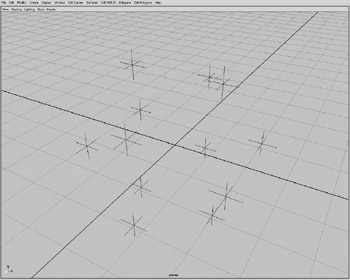
Figure 6.2: The locators in the viewport.

For purposes of clarity, we will now remap our vertex locator numbers , as seen in Figure 6.3.

On the CD  

The text for this script is found on the companion CD-ROM as /project_01/v03/buildPolyIcosohedron.mel.

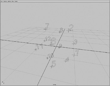
Figure 6.3: The remapped vertex numbers.

Now that our vertices are in the correct location, we need to build our individual faces. To create individual polygons in the Maya interface, we use the Polygon > Create Polygon tool.

An important aspect of creating polygonal faces is vertex order . In Maya, the normal of a face is defined on creation by the direction the vertices are created. As seen in Figure 6.4, if viewed along the normal, the vertices of a polygon proceed in a counterclockwise order.

Figure 6.4: Vertex creation order and normal direction.

If we start a new file, source and execute our script, we now have 12 locators corresponding to the 12 vertices of our icosahedron. We can now build each face using the Create Polygon tool, and turning on Point Snap to guarantee that each vertex will be placed on our newly created locators.

Following the rules for creating polygons, create 20 triangular faces in the following order:

Face 01: Vertex 01, Vertex 03, Vertex 02
Face 02: Vertex 01, Vertex 04, Vertex 03
Face 03: Vertex 01, Vertex 05, Vertex 04
Face 04: Vertex 01, Vertex 06, Vertex 05
Face 05: Vertex 01, Vertex 02, Vertex 06
Face 06: Vertex 02, Vertex 03, Vertex 08
Face 07: Vertex 03, Vertex 09, Vertex 08
Face 08: Vertex 03, Vertex 04, Vertex 09
Face 09: Vertex 04, Vertex 10, Vertex 09
Face 10: Vertex 04, Vertex 05, Vertex 10
Face 11: Vertex 05, Vertex 11, Vertex 10
Face 12: Vertex 05, Vertex 06, Vertex 11
Face 13: Vertex 06, Vertex 07, Vertex 11
Face 14: Vertex 06, Vertex 02, Vertex 07
Face 15: Vertex 02, Vertex 08, Vertex 07
Face 16: Vertex 12, Vertex 07, Vertex 08
Face 17: Vertex 12, Vertex 08, Vertex 09
Face 18: Vertex 12, Vertex 09, Vertex 10
Face 19: Vertex 12, Vertex 10, Vertex 11
Face 20: Vertex 12, Vertex 11, Vertex 07

This should give us something resembling Figure 6.5, 20 separate objects that together form the shape of an icosahedron.

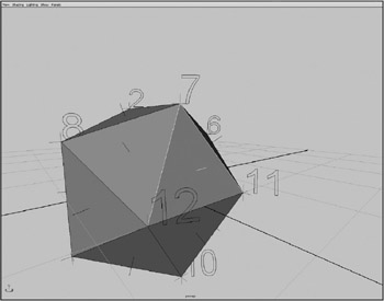
Figure 6.5: The separate objects that form the icosahedron.

So far, so good. We now have to put the creation of those polygons into the script. If we look in the History area of the Script Editor, we can see a series of polyCreateFacet commands. The command polyCreateFacet is the MEL command that creates polygonal faces. Each should look similar to Example 6.5.

Example 6.5: The results of creating a polygonal face.

 polyCreateFacet -ch on -tx 1 -s 1 -p 1 0 0.618034         -p 1 0 -0.618034 -p 0.618034 1 0 ;  // Result: polySurface1 polyCreateFace1 //  

One of the slightly illogical things Maya does when it gives feedback in the History area of the Script Editor is that it uses the short flags for each command, rather than the more informative long flag names . To decipher the flags, we can either refer to the online HTML documentation of MEL commands, or simply type help polyCreateFacet in the Script Editor. Doing so allows us to translate our command into that seen in Example 6.6. We have also cleaned up the command to add white space and readability.

Example 6.6: Putting the command into an easily readable format.

 polyCreateFacet         -constructionHistory on         -texture 1         -subdivision 1         -point 1 0 0.618034         -point 1 0 -0.618034         -point 0.618034 1 0         ; 

We can now replace the creation of the vertex locators in our script with 20 polyCreateFacet commands. In each, we will want to replace the numbers after each of the “point flags with the vector variables, in the same order we built the facets by hand. In Example 6.7, we see how the variables are used to build the first face.

On the CD  

The text for this script is found on the companion CD-ROM as /project_01/v04/buildPolyIcosohedron.mel.

Example 6.7: Using the variables in the creation of our polygons.

 polyCreateFacet         -constructionHistory off         -texture 1         -subdivision 1         -point ($vert_01.x) ($vert_01.y) ($vert_01.z)         -point ($vert_03.x) ($vert_03.y) ($vert_03.z)         -point ($vert_02.x) ($vert_02.y) ($vert_02.z)     ; 

We have chosen to turn off the construction history during the creation of our polygon faces because we have no need for the history, and having that history simply clutters the scene with unneeded nodes. As we will learn later, having these extra nodes does more than just add bloat to a file; they can actually slow down scripts when we have to navigate through the node connections of objects.

After adding the commands to create the 20 separate faces of our icosahedron, we can start a new file, source and execute our script, giving us essentially what we had before, but now created by the script.

Obviously, we don t want our icosahedron to be made of 20 separate pieces. We can select all the faces and from the Modeling menu select Polygon -> Combine to make one object of the individual polygons. If Construction History is on, we can look in the Hypergraph and see that the nodes that now make up the icosahedron still exist. Once we delete the construction history on the newly created icosahedron object, the nodes disappear. We can now look in the Script Editor history to find the commands for what we have just done.

The command to combine polygons is polyUnite . We can just copy the code for our polyUnite command, but alter the flag so that we do not create construction history, as seen in Example 6.8.

Example 6.8: Combining the individual faces into one object.

 polyUnite         -constructionHistory off         polySurface1         polySurface2         polySurface3         polySurface4         polySurface5         polySurface6         polySurface7         polySurface8         polySurface9         polySurface10         polySurface11         polySurface12         polySurface13         polySurface14         polySurface15         polySurface16         polySurface17         polySurface18         polySurface19         polySurface20         ; 

Now if we source and execute our script, unless it s a new scene, we get an error similar to that seen in Example 6.9.

Example 6.9: An example of the error that likely occurred.

  // Error: file: C:/Documents and Settings/Administrator   /My Documents/maya/scripts/TMC/chapter_06/  buildIcosohedron.mel line 284: No object matches     name: polySurface1 // 

This is due to the command using the explicit names polySurface1, polySurface2, and so forth. As we can see from looking at the Hypergraph, the new faces start with the name polySurface22. When we combined our faces into the icosahedron, it became polySurface21. Because of the way Maya handles naming new objects, there is no guarantee that, even if we explicitly assign a name to the polygon faces upon creation, we can know the names of the actual polygon objects the script creates. What we need to do is catch the name of an object as it is created and assign that captured name to a variable. We do this by enclosing the polyCreateFacet command in single forward quotes, and assigning it to a string variable, as seen in Example 6.10.

Example 6.10: Capturing the name of the created object.

 string $surf_01[] = `polyCreateFacet         -constructionHistory off         -texture 1         -subdivision 1         -point ($vert_01.x) ($vert_01.y) ($vert_01.z)         -point ($vert_03.x) ($vert_03.y) ($vert_03.z)         -point ($vert_02.x) ($vert_02.y) ($vert_02.z)         `         ; 

We use a string array variable because the polyCreateFacet command is designed to return not only the name of the object s transform node, but the nodes it creates when the command is used with Construction History turned on.

This idea, that Maya returns a single piece of information as an array, is the cause of many errors within scripts. While it is little more than an irritation when this occurs within a script, since it is a simple matter to add the [] to a variable to make it an array, it is a problem for global variables, since you cannot re-declare a variable of the same name as a different type. If you are unclear as to what type of data a command returns information as, simply attempt to assign the return data to a known type of variable, and if the return type differs , the resulting error will reveal what the return data type is.

Add this variable assignment, using $surf_01[] , $surf_02[] , and so on, to each of the polyCreateFacet commands. Now, we can use those variables in place of the explicit object names in the polyUnite command, as seen in Example 6.11.

Example 6.11: Using the captured names in the polyUnite command.

 polyUnite         -constructionHistory off         $surf_01         $surf_02         $surf_03         $surf_04         $surf_05         $surf_06         $surf_07         $surf_08         $surf_09         $surf_10         $surf_11         $surf_12         $surf_13         $surf_14         $surf_15         $surf_16         $surf_17         $surf_18         $surf_19         $surf_20         ; 

At this point we can now execute our script as many times as we want without errors and get a new icosahedron each time. We do have one last aspect of creating the icosahedron unresolved . An icosahedron has 12 vertices. Although it appears that our icosahedron has only 12, it actually has 60, which can be confirmed through the command polyEvaluate “vertex , a command that returns the number of vertices in a selected object. Although the polyUnite command combines the multiple objects into a single object, it does not unite any of the components. In the Maya interface we can use the Edit Polygons -> Merge Vertices command to merge all the overlapping vertices. The option settings for the Merge Vertices command are seen in Figure 6.6. We have to find a balance for the tolerance settings so that the overlapping vertices are merged, but not the neighbor vertices.

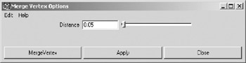
Figure 6.6: Merge Vertex Options box.

Successfully merging the vertices of a polygonal object is dependent upon the normals of an object. Because we put the effort into ensuring that all the normals of the polygons were created with the polyCreateFacet command, we should have no problems. The effort spent to create objects the right way often saves extra work and possible bugs later.

We can now harvest the resulting command from the Script Editor. Again, as we see in Example 6.12, an object is explicitly named in the command, polyMergeVertex . Actually, the object is not named, but rather its vertex components. For now, since we are essentially dealing with all the vertices as a single entity, we will keep our component handling simple. We will cover object components in depth in Project 6.3.

Example 6.12: The command to merge polygonal vertices.

 polyMergeVertex -d 0.05 -ch 0 polySurface21.vtx[0:59]; 

As in the case of the polyUnite command, we need to know the name of the newly created icosahedron to pass to the polyMergeVertex command. Create a variable to catch the result of the polyUnite command, as seen in Example 6.13. Notice again that the variable is an array, although we are capturing only a single element.

Example 6.13: Capturing the name of the polyUnite created object to a string variable.

 string $united_poly[] = `polyUnite                                  -constructionHistory off                                  $surf_01                                  $surf_02                                  $surf_03                                  $surf_04                                  $surf_05                                  $surf_06                                  $surf_07                                  $surf_08                                  $surf_09                                  $surf_10                                  $surf_11                                  $surf_12                                  $surf_13                                  $surf_14                                  $surf_15                                  $surf_16                                  $surf_17                                  $surf_18                                  $surf_19                                  $surf_20