MATRIX OPERATIONS | Six Sigma and Beyond: Statistics and Probability, Volume III

The power of matrix algebra becomes apparent when we explore the operations that are possible. The major operations are addition, subtraction, multiplication, and inversion. Many statistical operations can be done by knowing the basic rules of matrix algebra. Some matrix operations are now defined and illustrated .

ADDITION AND SUBTRACTION

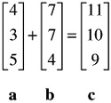
Two or more vectors can be added or subtracted provided they are of the same dimensionality. That is, they have the same number of elements. The following two vectors are added:

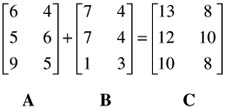
Similarly, matrices of the same dimensionality may be added or subtracted. The following two 3-by-2 matrices are added:

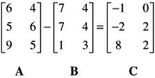
Now, B is subtracted from A:

MULTIPLICATION

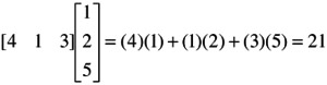
To obtain the product of a row vector by a column vector, corresponding elements of each are multiplied and then added. For example, the multiplication of a ' by b , each consisting of three elements, is:

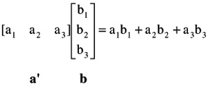
Note that the product of a row by a column is a single number called a scalar. This is why the product of a row by a column is referred to as the scalar product of vectors. Here is a numerical example:

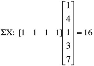
Scalar products of vectors are very frequently used in statistical analysis. For example, to obtain the sum of the elements of a column vector it is premultiplied by a unit row vector of the same dimensionality. Thus,

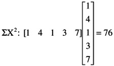
The sum of the squares of a column vector is obtained by premultiplying the vector by its transpose:

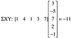
Similarly, the sum of the products of X and Y is obtained by multiplying the row of X by the column of Y, or the row of Y by the column of X.

Scalar products of vectors are used frequently in dealing with multiple regression, discriminant analysis, multivariate analysis of variance, and canonical analysis.

Instead of multiplying a row vector by a column vector, one may multiply a column vector by a row vector. The two operations are entirely different from each other. It was shown above that the former results in a scalar. The latter operation, on the other hand, results in a matrix. This is why it is referred to as the matrix product of vectors. For example:

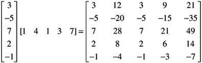
Note that each element of the column is multiplied, in turn , by each element of the row to obtain one element of the matrix. The product of the first element of the column by the row elements becomes the first row of the matrix. Those of the second element of the column by the row become the second row of the matrix, and so forth. Thus, the matrix product of a column vector of k elements is a k — k matrix.

Matrix multiplication is done by multiplying rows by columns . An example is easier than verbal explanation. Suppose we want to multiply two matrices, A and B , to produce the product matrix C :

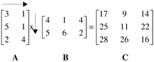
Following the rule of scalar product of vectors, we multiply and add as follows (follow the arrows):

(3)(4) + (1)(5) = 17	(3)(1) + (1)(6) = 9	(3)(4) + (1)(2) = 14
(5)(4) + (1)(5) = 25	(5)(1) + (1)(6) = 11	(5)(4) + (1)(2) = 22
(2)(4) + (4)(5) = 28	(2)(1) + (4)(6) = 26	(2)(4) + (4)(2) = 16

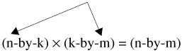
From the foregoing illustration, it may be discerned that in order to multiply two matrices it is necessary that the number of columns of the first matrix be equal to the number of rows of the second matrix. This is referred to as the conformability condition. Thus, for example, an n-by-k matrix can be multiplied by a k-by-m matrix because the number of rows of the first (k) is equal to the number of rows of the second (k). In this context, the k's are referred to as the "interior" dimensions; n and m are referred to as the "exterior" dimensions.

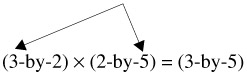
Two matrices are conformable when they have the same "interior" dimensions. There are no restrictions on the "exterior" dimensions when two matrices are multiplied. It is useful to note that the "exterior" dimensions of two matrices being multiplied become the dimensions of the product matrix. For example, when a 3-by-2 matrix is multiplied by a 2-by-5 matrix, a 3-by-5 matrix is obtained:

In general,

A special case of matrix multiplication often encountered in statistical work is the multiplication of a matrix by its transpose to obtain a matrix of raw score or deviation Sums of Squares and Cross Products (SSCP). Assume that there are n subjects for whom measures on k variables are available. In other words, assume that the data matrix, X, is an n-by-k. To obtain the raw score SSCP, calculate X'X. Here is a numerical example:

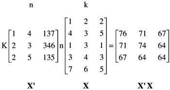
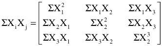
In statistical symbols, X'X is

Using similar operations, one may obtain deviation SSCP matrices. Such matrices are used frequently in statistical calculations of advanced methodologies.

A matrix can be multiplied by a scalar: each element of the matrix is multiplied by the scalar. Suppose, for example, we want to calculate the mean of each of the elements of a matrix of sums of scores. Let N = 10. The operation is

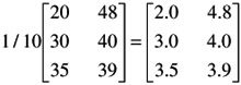
Each element of the matrix is multiplied by the scalar 1/10.

A matrix can also be multiplied by a vector. The first example given below is premultiplication by a vector; the second is postmultiplication:

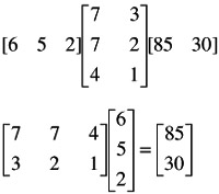
Note that in the latter example, (2-by-3) — (3-by-1) becomes (2-by-1). This sort of multiplication of a matrix by a vector is done very frequently in multiple regression.

Thus far, nothing has been said about the operation of division in matrix algebra. In order to show how this is done it is necessary first to discuss some other concepts, to which we now turn.

DETERMINANTS

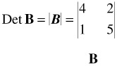
A determinant is a certain numerical value associated with a square matrix. The determinant of a matrix is indicated by vertical lines instead of brackets. For example, the determinant of a matrix B is written

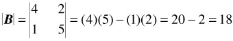
The calculation of the determinant of a 2 — 2 matrix is very simple: it is the product of the elements of the principal diagonal minus the product of the remaining two elements. For the above matrix,

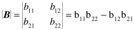
or, symbolically,

The calculation of determinants for larger matrices is quite tedious and will not be shown here (see references listed at the end of this appendix). In any event, matrix operations are most often done with the aid of a computer. The purpose here is solely to indicate the role played by determinants in some applications of statistical analysis.

APPLICATIONS OF DETERMINANTS

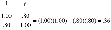
To give the flavor of the place and usefulness of determinants in statistical analysis we turn first to two simple correlation examples. Suppose we have two correlation coefficients, r _y1 , and r _y2 , calculated between a dependent variable, Y, and two variables, 1 and 2. The correlations are r _y1 = .80 and r _y2 = .20. We set up two matrices that express the two relations, but this is done immediately in the form of determinants, whose numerical values are calculated:

and

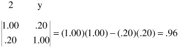
The two determinants are .36 and .96. Now, to determine the percentage of variance shared by y and 1 and by y and 2, square the r's:

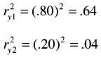
Subtract each of these from 1.00: 1.00 - .64 = .36, and 1.00 - .04 = .96. These are the determinants just calculated. They are 1 - r ² , or the proportions of the variance not accounted for.

As an extension of the foregoing demonstration, it may be shown how the squared multiple correlation, R ² , can be calculated with determinants:

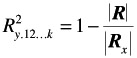
where R is the determinant of the correlation matrix of all the variables, that is, the independent variables as well as the dependent variable; R _x is the determinant of the correlation matrix of the independent variables. From the foregoing it can be seen that the ratio of the two determinants indicates the proportion of variance of the dependent variable, Y, not accounted by the independent variables, X's. The ratio of two determinants is also frequently used in multivariate analyses dealing with Wilks' A.

Another important use of determinants is related to the concept of linear dependencies, to which we now turn.

LINEAR DEPENDENCE

Linear dependence means that one or more vectors of a matrix, rows or columns, are a linear combination of other vectors of the matrix. The vectors a' = [3 1 4] and b' = [6 2 8] are dependent since 2 a' = b' . If one vector is a function of another in this manner, the coefficient of correlation between them is 1.00. Dependence in a matrix can be defined by reference to its determinant. If the determinant of the matrix is zero it means that the matrix contains at least one linear dependency. Such a matrix is referred to as being singular. For example, calculate the determinant of the following matrix:

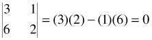
The matrix is singular, that is, it contains a linear dependency. Note that the values of the second row are twice the values of the first row.

A matrix with a determinant other than zero is referred to as being nonsingular. The notions of singularity and nonsingularity of matrices play very important roles in statistical analysis, especially in the analysis of multicollinearity. As is shown below, a singular matrix has no inverse.

We turn now to the operation of division in matrix algebra, which is presented in the context of the discussion of matrix inversion.

MATRIX INVERSE

Recall that the division of one number into another number amounts to multiplying the dividend by the reciprocal of the divisor:

For example, 12/4 = 12(1/4) = (12)(.25) = 3. Analogously, in matrix algebra, instead of dividing a matrix A by another matrix B to obtain matrix C , we multiply A by the inverse of B to obtain C . The inverse of B is written B ^- ¹ . Suppose, in ordinary algebra, we had ab = c, and we wanted to find b. We would write

In matrix algebra, we write

B = A ^-1 C

(Note that C is premultiplied by A ^-1 and not postmultiplied. In general, A ^-1 C ‰ CA ^-1 .)

The formal definition of the inverse of a square matrix is: Given A and B , two square matrices, if AB = I , then A is the inverse of B .

Generally , the calculation of the inverse of a matrix is very laborious and, therefore, error prone. This is why it is best to use a computer program for such purposes (see below). Fortunately, however, the calculation of the inverse of a 2 — 2 matrix is very simple, and is shown here for three reasons:

It affords an illustration of the basic approach to the calculation of the inverse.
It affords the opportunity to show the role played by the determinant in the calculation of the inverse.
Inverses of 2 — 2 matrices are frequently calculated in some applications of statistical tools and especially in multivariate analysis.

In order to show how the inverse of a 2 — 2 matrix is calculated, it is necessary first to discuss briefly the adjoint of such a matrix. This is shown in reference to the following matrix:

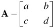
The adjoint of A is:

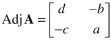
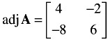
Thus, to obtain the adjoint of a 2 — 2 matrix, interchange the elements of its principal diagonal (a and d in the above example), and change the signs of the other two elements (b and c in the above example). Now the inverse of a matrix A is:

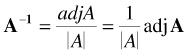
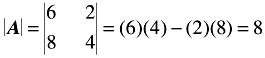
where A is the determinant of A . The inverse of the following matrix, A , is now calculated.

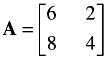
First, calculate the determinant of A :

Second, form the adjoint of A :

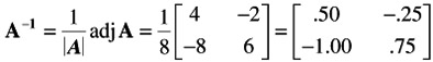
Third, multiply the adj A by the reciprocal of A to obtain the inverse of A .

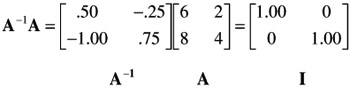
It was mentioned earlier that A ^-1 A = I . For the present example,

It was said above that a matrix with a determinant of zero is singular. From the foregoing demonstration of the calculation of the inverse, it should be clear that a singular matrix has no inverse. Although one does not generally encounter singular matrices, an unwary researcher may introduce singularity in the treatment of the data. For example, suppose that a test battery consisting of five subtests is used to predict a given criterion. If, under such circumstances, the researcher uses not only the results on the five subtests but also a total test, obtained as the sum of the five subtests, he or she has introduced a linear dependency (see above), thereby rendering the matrix singular; similarly, when one uses tests on two scales as well as the differences between them in the same matrix. Other situations when one should be on guard not to introduce linear dependencies in a matrix occur when coded vectors are used to represent categorical variables.

It is realized that this brief introduction to matrix algebra cannot serve to demonstrate its great power and elegance . To do this, it would be necessary to use matrices with dimensions larger than the ones used here for simplicity of presentation. To begin to appreciate the power of matrix algebra, it is suggested that you think of the large data matrices frequently encountered in product development of any large corporation. Using matrix algebra, one can manipulate and operate upon large matrices with relative ease, when ordinary algebra will simply not do. For example, when in multiple regression analysis only two independent variables are used, it is relatively easy to do the calculations by ordinary algebra. But with increasing numbers of independent variables, the use of matrix algebra for the calculation of multiple regression analysis becomes a must. And in addition, matrix algebra is the language of linear structural equation models and multivariate analysis. In short, to understand and be able to intelligently apply these methods , it is essential that you develop a working knowledge of matrix algebra. It is therefore strongly suggested that you do a serious review of some of the references already mentioned in this appendix. Furthermore, it is suggested that you learn to use computer programs when you have to manipulate relatively large matrices. Of the various computer programs for matrix manipulations, one of the best and most versatile is the MATRIX program of the SAS package, followed by SPSS and Minitab.