NORMAL APPROXIMATION OF BINOMIAL

Binomial probability distribution:

with mean: ¼ = np and variance: ƒ ² = npq.

Assumptions:

Neither of the binomial probabilities p or q = 1-p is near zero.
Sample size n is "sufficiently" large (how large depends upon p).
The binomial distribution appears nearly symmetric about the mean in Figure 16.26.

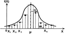
Figure 16.26: A typical binomial distribution.

Issues: Binomial lower limit is zero; normal is - ˆ . Binomial is discrete of cell width, W _c ; normal is continuous random variable.

Accuracy improves if:

Sample size n increases , or
Probability approaches p = 1/2

Certain n and p combinations provide a good approximation for modeling of a binomial population by a normal distribution. Confining our approximation to the interval: ¼ ± 3 ƒ requires only that the binomial products np > 5 and nq > 5. These products yield binomial distributions which are nearly symmetric about mean ¼ = np; and have a variance ƒ ² = npq.

It is this symmetry about the mean that allows us to approximate the binomial distribution as a normal distribution and thereby use the tabulated values to determine its probabilities. Standardized random variables for the binomial distribution are:

After defining the binomial distribution problem, the probability being sought can be determined from the table of standardized normal distribution in the form: p (Z ₁ Z Z ₂ ). As a rule of thumb, the following minimum sample sizes may be used for a normal distribution model to approximate a binomial population.

p = 0.5	n 30
p = 0.4 or 0.6	n 50
p = 0.3 or 0.7	n 80
p = 0.2 or 0.8	n 200
p = 0.1 or 0.9	n 600
p = 0.05 or 0.95	n 1400

Example 1

Given: A supplier produces a special order of 280 electronic instruments, but past history has shown that 10% of this company's products are defective.

Find: If the number of defects is assumed to be binomially distributed, compute the chance that number of defects does not exceed 23 instruments. (The value 23 is a threshold.)

Statistics:

p = 0.10, q = 0.90, ¼ = np = 28 > 5, nq = 252 >> 5, ƒ = (npq) ^1/2 = 5.0

Direct application of binomial distribution

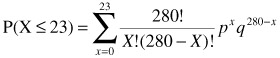
While this is the true calculation, it is very time-consuming , and tables do not exist to condense the labor involved. As a result we use the approximation approach by applying the normal distribution approximation as follows . (In a pictorial format it is shown in Figure 16.27).

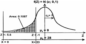
Figure 16.27: Normal distribution approximation.

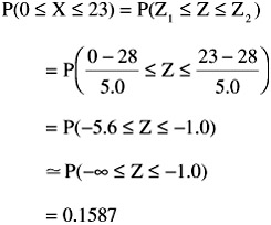
Therefore, there is a 15.9% chance that no more than 23 instruments will not "meet spec."

Some general comments on continuity correction:

The normal distribution is based on a continuous RV while the binomial distribution is based on a discrete countable integer RV grouped into cells of a specified width, C _w .
The range interval for the continuous normal distribution is from - ˆ to + ˆ , whereas the binomial distribution is on countable integers (items) ranging from 0 to n.
A continuity correction is applied to the discrete cells to improve the accuracy of the approximation.
The correction consists of:
1. subtract 1/2-cell width from the lower limit and
2. add 1/2-cell width to the upper limit
These limits in standardized form are:

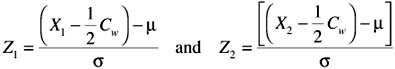
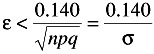
When using the continuity correction, always remember that the error for the normal distribution to approximate the binomial distribution never exceeds:

Example 2

Given: A manufacturer produces a special order of 280 electronic instruments, but past history has shown that 10% of the instruments that it produces are defective.

Find: if the number of defects is assumed to be binomially distributed, compute the chance that exactly 28 defective instruments are manufactured.

Statistics: p = 0.10, q = 0.90, ¼ = np = 28 > 5, n q = 252 >> 5, ƒ = (npq) ^1/2 = 5.0, cell width = 1 product, 1/2-cell = 0.5.

Solution:

Direct application of binomial distribution:

Normal distribution approximation:

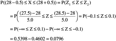
Therefore, there is a 7.96% possibility of producing exactly 28 defects.

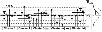
Figure 16.28: Mean of the means.