MULTIVARIATE ANALYSIS OF VARIANCE (MANOVA)

MANOVA is an extension of univariate analysis of variance designed to simultaneously test differences among groups on multiple dependent variables . Several tests have been proposed for this purpose. Probably the most widely used among them is a test of Wilks' . That is, a test of (shown below) serves as an overall test of the null hypothesis of the equality of mean vectors of two or more groups.

In an earlier section, was discussed in detail in the context of DA, though the test of significance for was not shown. A question that naturally arises is: Since may be obtained in both DA and MANOVA, in what way do these approaches differ ? Issues of classification to which DA but not MANOVA may be applied aside, it was said earlier that some researchers treat MANOVA and DA as interchangeable when the concern is the study of group differences. But other researchers recommend that MANOVA be applied first in order to determine whether there are overall significant differences among the groups. This is accomplished by testing . If the null hypothesis is rejected, it is recommended that DA be used to identify the variables on which the groups differ to the greatest extent and the nature of the dimensions on which they differ.

It was stated above that when more than two groups are being studied, more than one discriminant function is obtained. In such situations, the test of still refers to overall differences among the groups. But if it is found that is statistically significant, it may turn out that only one or two discriminant functions are statistically significant, even though the data allow the calculation of a greater number of such functions.

TESTING THE ASSUMPTIONS OF MULTIVARIATE ANALYSIS

As we already have discussed several times, data are the life blood of any statistical analysis. However, the data must be appropriate and applicable for the type of analysis that we want to conduct. The introduction to this book mentioned some of the preliminary steps in preparing data for analysis. Here we are going to address the final step in examining the data, which involves testing the assumptions underlying multivariate analysis. The need to test the statistical assumptions is increased in multivariate applications because of two characteristics of multivariate analysis. First, the complexity of the relationships, owing to the typical use of a large number of variables, makes the potential distortions and biases more potent when the assumptions are violated. This is particularly true when the violations compound to become even more detrimental than if considered separately. Second, the complexity of the analyses and of the results may mask the "signs" of assumption violations apparent in the simpler univariate analyses. In almost all instances, the multivariate procedures will estimate the multivariate model and produce results even when the assumptions are severely violated. Thus, the experimenter must be aware of any assumption violations and the implications they may have for the estimation process or the interpretation of the results.

ASSESSING INDIVIDUAL VARIABLES VERSUS THE VARIATE

Multivariate analysis requires that the assumptions underlying the statistical techniques be tested twice: first for the separate variables, akin to the tests of assumption for univariate analyses, and second for the multivariate model variate, which acts collectively for the variables in the analysis and thus must meet the same assumptions as individual variables do.

Normality

The most fundamental assumption in multivariate analysis is normality, referring to the shape of the data distribution for an individual metric variable and its correspondence to the normal distribution, the benchmark for statistical methods . If the variation from the normal distribution is sufficiently large, all resulting statistical tests are invalid because normality is required for use of the F and t statistics. Both the univariate and the multivariate statistical methods discussed in this volume are based on the assumption of univariate normality, with the multivariate methods also assuming multivariate normality. Univariate normality for a single variable is easily tested, and a number of corrective measures are possible, as shown later. In a simple sense, multivariate normality (the combination of two or more variables) means that the individual variables are normal in a univariate sense and that their combinations are also normal. Thus, if a variable is multivariate normal, it is also univariate normal. However, the reverse is not necessarily true (two or more univariate normal variables are not necessarily multivariate normal). Thus a situation in which all variables exhibit univariate normality will help gain, although not guarantee, multivariate normality. Multivariate normality is more difficult to test, but some tests are available for situations in which the multivariate technique is particularly affected by a violation of this assumption. In this text, we focus on assessing and achieving univariate normality for all variables and address multivariate normality only when it is especially critical. Even though large sample sizes tend to diminish the detrimental effects of nonnormality, the researcher should assess the normality for all variables included in the analysis.

Graphical Analyses of Normality

The simplest diagnostic test for normality is a visual check of the histogram that compares the observed data values with a distribution approximating the normal distribution. Although appealing because of its simplicity, this method is problematic for smaller samples, where the construction of the histogram (e.g., the number of categories or the width of categories) can distort the visual portrayal to such an extent that the analysis is useless. A more reliable approach is the normal probability plot, which compares the cumulative distribution of actual data values with the cumulative distribution of a normal distribution. The normal distribution forms a straight diagonal line, and the plotted data values are compared with the diagonal. If a distribution is normal, the line representing the actual data distribution closely follows the diagonal.

Figure 11.2 shows several normal probability plots and the corresponding univariate distribution of the variable. One characteristic of the distribution's shape, the kurtosis, is reflected in the normal probability plots. Kurtosis refers to the "peakedness" or " flatness " of the distribution compared with the normal distribution. When the line falls below the diagonal, the distribution is flatter than expected. When it goes above the diagonal, the distribution is more peaked than the normal curve. For example, in the normal probability plot of a peaked distribution (Figure 11.2d), we see a distinct S-shaped curve. Initially the distribution is flatter, and the plotted line falls below the diagonal. Then the peaked part of the distribution rapidly moves the plotted line above the diagonal, and eventually the line shifts to below the diagonal again as the distribution flattens. A nonpeaked distribution has the opposite pattern (Figure 11.2c). Another common pattern is a simple arc, either above or below the diagonal, indicating the skewness of the distribution. A negative skewness (Figure 11.2e) is indicated by an arc below the diagonal, whereas an arc above the diagonal represents a positively skewed distribution (Figure 11.2f). An excellent source for interpreting normal probability plots, showing the various patterns and interpretations, is Daniel and Wood (1980). These specific patterns not only identify nonnormality but also tell us the form of the original distribution and the appropriate remedy to apply.

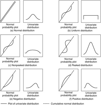
Figure 11.2: Normal probability plots and corresponding univariate distributions.

Statistical Tests of Normality

In addition to examining the normal probability plot, one can also use statistical tests to assess normality. A simple test is a rule of thumb based on the skewness and kurtosis values (available as part of the basic descriptive statistics for a variable computed by all statistical programs). The statistic value (z) for the skewness value is calculated as:

where N is the sample size . A z value can also be calculated for the kurtosis value using the following formula:

If the calculated z value exceeds a critical value, then the distribution is nonnormal in terms of that characteristic. The critical value is from a z distribution, based on the significance level we desire . For example, a calculated value exceeding ±2.58 indicates we can reject the assumption about the normality of the distribution at the .01 probability level. Another commonly used critical value is t 1.96, which corresponds to a .05 error level. (Specific statistical tests are also available in SPSS, SAS, BMDP, and most other programs. The two most common are the Shapiro-Wilks test and a modification of the Kolmogorov-Smirnov test. Each calculates the level of significance for the differences from a normal distribution. The experimenter should always remember that tests of significance are less useful in small samples [fewer than 30] and quite sensitive in large samples [exceeding 1,000 observations]. Thus, the researcher should always use both the graphical plots and any statistical tests to assess the actual degree of departure from normality.)

Remedies for Nonnormality

A number of data transformations available to accommodate nonnormal distributions are discussed later in the chapter. This chapter confines the discussion to univariate normality tests and transformations. However, when we examine other multivariate methods, such as multivariate regression or multivariate analysis of variance, we discuss tests for multivariate normality as well. Moreover, many times when nonnormality is indicated, it is actually the result of other assumption violations; therefore, remedying the other violations eliminates the nonnormality problem. For this reason, the researcher should perform normality tests after or concurrently with analyses and remedies for other violations. (Those interested in multivariate normality should see Johnson and Wichern [1982] and Weisberg [1985].)

Homoscedasticity

Homoscedasticity is an assumption related primarily to dependence relationships between variables. It refers to the assumption that dependent variable(s) exhibit equal levels of variance across the range of predictor variable(s). Homoscedasticity is desirable because the variance of the dependent variable being explained in the dependence relationship should not be concentrated in only a limited range of the independent values. Although the dependent variables must be metric, this concept of an equal spread of variance across independent variables can be applied when the independent variables are either metric or nonmetric. With metric independent variables, the concept of homoscedasticity is based on the spread of dependent variable variance across the range of independent variable values, which is encountered in techniques such as multiple regression. The same concept also applies when the independent variables are nonmetric. In these instances, such as are found in ANOVA and MANOVA, the focus now becomes the equality of the variance (single dependent variable) or the variance/covariance matrices (multiple independent variables) across the groups formed by the nonmetric independent variables. The equality of variance/covariance matrices is also seen in discriminant analysis, but in this technique the emphasis is on the spread of the independent variables across the groups formed by the nonmetric dependent measure. In each of these instances, the purpose is the same: to ensure that the variance used in explanation and prediction is distributed across the range of values, thus allowing for a "fair test" of the relationship across all values of the nonmetric variables.

In most situations, we have many different values of the dependent variable at each value of the independent variable. For this relationship to be fully captured, the dispersion (variance) of the dependent variable values must be equal at each value of the predictor variable. Most problems with unequal variances stem from one of two sources. The first source is the type of variables included in the model. For example, as a variable increases in value (e.g., units ranging from near zero to millions), there is naturally a wider range of possible answers for the larger values.

The second source results from a skewed distribution that creates heteroscedasticity, In Figure 11.3a, the scatterplots of data points for two variables (V ₁ and V ₂ ) with normal distributions exhibit equal dispersion across all data values (i.e., homoscedasticity). However, in Figure 11.3b, we see unequal dispersion (heteroscedasticity) caused by skewness of one of the variables (V ₃ ). For the different values of V ₃ , there are different patterns of dispersion for V ₁ . This will cause the predictions to be better at some levels of the independent variable than at others. Violating this assumption often makes hypothesis tests either too conservative or too sensitive.

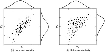
Figure 11.3: Scatterplots of homoscedastic and heteroscedastic relationships.

The effect of heteroscedasticity is also often related to sample size, especially when examining the variance dispersion across groups. For example, in ANOVA or MANOVA, the impact of heteroscedasticity on the statistical test depends on the sample sizes associated with the groups of smaller and larger variances. In multiple regression analysis, similar effects would occur in highly skewed distributions where there were disproportionate numbers of respondents in certain ranges of the independent variable.

Graphical Tests of Equal Variance Dispersion

The test of homoscedasticity for two metric variables is best examined graphically. The most common application of this form of assessment occurs in multiple regression, which is concerned with the dispersion of the dependent variable across the values of the metric independent variables. Because the focus of regression analysis is on the regression variate, the graphical plot of residuals is used to reveal the presence of homoscedasticity (or its opposite, heteroscedasticity). The earlier discussion of residual analysis details these procedures. Boxplots work well to represent the degree of variation between groups formed by a categorical variable. The length of the box and the whiskers each portray the variation of data within that group. A typical boxplot is shown in Figure 11.4.

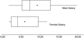
Figure 11.4: A typical comparison of side-by-side boxplots.

Statistical Tests for Homoscedasticity

The statistical tests for equal variance dispersion relate to the variances within groups formed by nonmetric variables. The most common test, the Levene test, can be used to assess whether the variances of a single metric variable are equal across any number of groups. If more than one metric variable is being tested, so that the comparison involves the equality of variance/covariance matrices, the Box's M test is applicable. The Box's M is a statistical test for the equality of the covariance matrices of the independent variables across the groups of the dependent variable. If the statistical significance is greater than the critical level (.01), then the equality of the covariance matrices is supported. If the test shows statistical significance, then the groups are deemed different and the assumption is violated. The Box's M test is available in both multivariate analysis of variance and discriminant analysis.

Remedies for Heteroscedasticity

Heteroscedastic variables can be remedied through data transformations similar to those used to achieve normality. As mentioned earlier, many times heteroscedasticity is the result of nonnormality of one of the variables, and correction of the nonnormality also remedies the unequal dispersion of variance.

Linearity

An implicit assumption of all multivariate techniques based on correlational measures of association, including multiple regression, logistic regression, factor analysis, and structural equation modeling, is linearity. Because correlations represent only the linear association between variables, nonlinear effects will not be represented in the correlation value. This results in an underestimation of the actual strength of the relationship. It is always prudent to examine all relationships to identify any departures from linearity that may impact the correlation.

Identifying Nonlinear Relationships

The most common way to assess linearity is to examine scatterplots of the variables and to identify any nonlinear patterns in the data. An alternative approach is to run a simple regression analysis and to examine the residuals. The residuals reflect the unexplained portion of the dependent variable; thus, any nonlinear portion of the relationship will show up in the residuals. The examination of residuals can also be applied to multiple regression, where the researcher can detect any nonlinear effects not represented in the regression variate. If a nonlinear relationship is detected , the most direct approach is to transform one or both variables to achieve linearity.