MEASURES OF DISPERSION

Measures of process dispersion portray the amount of spread or variation in a data set. The range and standard deviation are two measures of dispersion. The range is used for small samples ( n < 8). The standard deviation is used for large samples ( n > 8).

Measures of dispersion aid in the interpretation of the mean. The mean gives the locations of the sample (as a group ) but does not represent each measurement equally. Measures of dispersion describe how well the mean represents each measurement. When the range is large, the mean is a relatively poor estimate for members of the sample that are far from the mean (see Figure 4.5). When the range is small, the mean is a relatively good estimate for all members of the sample (see Figure 4.5).

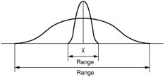
Figure 4.5: A comparison of the average and the range.

RANGE

The simplest measure of dispersion is the range ( R ), The range of a sample is calculated as the difference between the largest and the smallest value. The difference is actually the distance between the largest and smallest values. The closer these values are, the smaller the range will be.

Steps for Calculating the Range of a Data Set

Below are measurements (in inches) of holes drilled by a machine. To calculate the range:

1.9

1.5

2

2.5

2.1

2.4

• Find the largest and the smallest value (1.5 and 2.5).

• Subtract the smallest value from the largest value (2.5 - 1.5 = 1). The range of diameters of holes drilled by the machine is 1 inch.

Although the machine drills 2.7-inch-diameter holes on the average, it is unsatisfactory because the range is so large. If the range were reduced from 1 to 0 inches ( R = 0), this would mean that there is no variation. All of the diameters would measure 2.7 inches.

STANDARD DEVIATION

The standard deviation is a measure of variation that is needed to describe the spread of populations. The range is a statistic that is limited to simple data because it requires a known largest and smallest value. These values are unknown for a population because the population is an estimated distribution (see Figure 4.6).

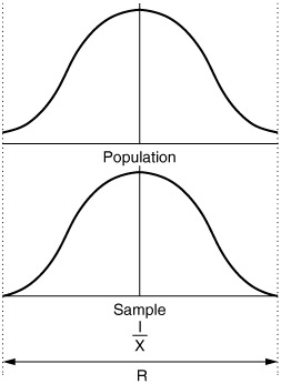
Figure 4.6: A comparison of population and sample.

The normal distribution has a curvature that slopes away from the mean. As the curve extends from the mean, the curve changes distribution. The precise point at which the curve changes directions is called the inflection point (see Figure 4.7). The standard deviation is the distance from the mean to the inflection point of the curve. The standard deviation is extremely valuable for describing the spread of a population because as the spread of the distribution increases, the distance to the inflection point increases .

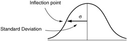
Figure 4.7: The relationship of the inflection point and the standard deviation.

The sample standard deviation is represented by s, and the corresponding population standard deviation, by the Greek lowercase sigma ( ƒ ).

Steps for Calculating the Sample Standard Deviation(s) for a Data Set

The formula for the standard deviation is as follows :

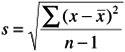
where

	=	square root
x	=	value
n - 1	=	degrees of freedom
	=	mean
& pound ;	=	the sum of
n	=	number of values

To calculate the standard deviation(s) for the following data set:

9

13

12

10

8

10

1. Calculate the mean (Xbar) of the data set:

   X bar	=	9 + 13 + 12 + 10 + 8 + 10 = 62; 62 · 6=10.33
   X bar	=	10.33

2. Set up a table (see Table 4.1) with the appropriate headings and perform the calculations necessary to determine X - X bar and ( X - X bar) ² .

   Table 4.1: Calculations for the Standard Deviation

   Value	X - X bar	( X - X bar) 2
   9	-1.33	1.77
   13	2.67	7.13
   12	1.67	2.79
   10	-0.33	0.11
   8	-2.33	5.43
   10	-0.33	0.11
   		17.34

3. Calculate the standard deviations of the data set. (Using a typical hand held calculator, the steps in Figure 4.8 are taken to solve the standard deviation.)

   
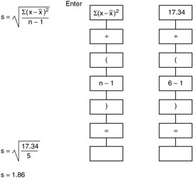
   Figure 4.8: Steps in calculating the standard deviation using a handheld calculator.

In general, most of the values should be within 1.86 of the mean.

This method demonstrates how the formula works. However, with a statistical calculator and a frequency distribution, the standard deviation can be determined much more easily because the numbers may be entered directly into the memory of the calculator without having to do the intermediate steps. To demonstrate that, we proceed with an example.

Steps for Calculating the Mean and Standard Deviation with a Statistical Calculator (Sharp Series)

To calculate the standard deviation( s ) and the mean ( X bar) of the data set below, follow these steps (see Figure 4.9):

Value	6	8	10	12	15
Frequency	1	1	8	2	1

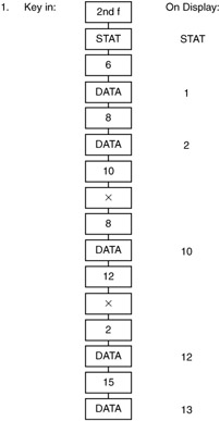
Figure 4.9: Calculating standard deviation using a statistical calculator (Sharp series).

1. To find the mean,

   Key in: < x bar>

   On Display:

   10.230769

2. To find the standard deviation,

   Key in: S	On Display:	2.0878157
   	(make sure to use the s button, not the ƒ button)

In addition,

• To set the calculator into the statistical mode, press the 2ndf and STAT keys, and "STAT" will appear in the upper part of the display.

• To remove past values, press the 2ndf and STAT keys. Then reset with 2ndf and STAT to put in a new set of values.

• The display will show "E" when an error has been made. An error can be caused by calculations made that are beyond the capacity of the calculator. Errors can be removed by the ON/C key.