SHORT-RUN CONTROL CHARTS FOR ATTRIBUTE DATA

To resolve many of the problems associated with applying SPC to short production runs when dealing with attribute data, several modified control charts have been developed. The rules for their application are exactly those of the traditional SPC and may be found in Chapters 9 and 10.

Because all the charts follow the same pattern and are very easy to do, we will provide the general formulas to calculate the limits and the plotting points without an extensive discussion. For more information, see Duncan (1986), Burr (1976), and Pyzdek (1989, 1992). All attribute charts have the following characteristics:

Center line is always 0.
Upper control limit is always +3.
Lower control limit is always -3.

SHORT-RUN NP

Plot Point. The plot point formula is derived in a similar manner to that for the short-run Xbar chart. The actual number of nonconforming units found (np) is coded by first subtracting the expected average (target npbar), then dividing this difference by the standard deviation (similar to calculating Z scores).

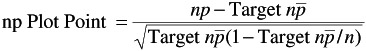
Assumptions. In addition to requiring a constant subgroup size , the short-run np chart assumes that the process output data follows a binomial distribution. The subgroup size used for each part number should be large enough to expect an average of at least two nonconforming units per subgroup.

SHORT-RUN P

Plot Point. The plot point formula is derived in a similar manner to the short-run Xbar chart. The number of nonconforming units found in the subgroup ( np ) is divided by the subgroup size ( n ) to calculate the percentage of nonconforming units ( p ) in the subgroup. This subgroup percentage is coded by first subtracting the expected average (target pbar), then dividing this difference by the standard deviation. This is very similar to the process of calculating Z scores.

Assumptions. The short-run p chart assumes that the process output data follow a binomial distribution. The subgroup size used for each part number should be large enough to expect an average of at least two nonconforming units per subgroup.

SHORT-RUN C

Plot Point. The plot point formula is derived in a similar manner to that for the short-run np chart. The actual number of nonconformities found ( c ) is coded by first subtracting the expected average (target cbar), then dividing this difference by the standard deviation (the square root of target cbar). This is very similar to the process of calculating Z scores.

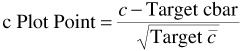
Assumptions. In addition to requiring a constant subgroup size, the short-run c chart assumes that the process output data follow a Poisson distribution. The subgroup size used for each part number should be large enough to expect an average of at least two nonconformities per subgroup.

SHORT-RUN U

Plot Point. The plot point formula is derived in a similar manner to that for the short-run p chart. The number of nonconformities found in the subgroup (c) is divided by the subgroup size ( n ) to determine the average number of nonconformities per unit ( u ) in the subgroup.

This u value is coded by first subtracting the expected average number of nonconformities (target ubar), then dividing this difference by the standard deviation (the square root of target ubar divided by ( n ). This is very similar to the process of calculating Z scores.

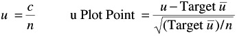
Assumptions. The short-run u chart assumes that the process output follows a Poisson distribution. The subgroup size used for each part number should be large enough to expect an average of at least two nonconformities per subgroup.