USEFUL CONCEPTS FOR FINANCIAL DECISIONS
THE MODIFIED DUPONT FORMULA
The duPont system of financial analysis combines profit margin and asset turnover to produce the return on assets. The modified version brings financial leverage into the equation to produce return on equity as well. The formulas are:
-
Asset Turnover — Return on Sales = Return on Assets
Sales/Assets — Profit/Sales = Profit/Assets
-
Return on Assets — Financial Leverage = Return on Equity
Profit/Assets — Assets/(Equity —) = Profit/Equity
A visual approach to duPont's concept is shown in Figure 15.2.
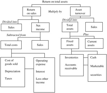
Figure 15.2: A pictorial approach of DuPont's formula.
BREAKEVEN ANALYSIS
The breakeven point for a business is that volume of sales at which the revenues equal the expenses. Above that point lie glory and profit; below lie infamy and loss. At least that is the theory. In real life, it is very difficult to calculate a breakeven point because the expenses of most businesses do not fit comfortably into just a fixed or variable category. Breakeven analysis can be done visually using a graph like the one in Figure 15.3, or mathematically.
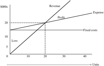
Figure 15.3: Breakeven analysis.
Profit = Sales - Fixed Costs - Variable Costs
If Fixed Costs = $12,000 and Variable Costs = 40% of Sales, then
Profit = Sales - $12,000 - .4*Sales
or Profit = .6*Sales - $12,000
At breakeven, profit will be 0, therefore 0 = .6*Sales - 12,000 and Sales = $12,000/.6 = $20,000 at that point.
CONTRIBUTION MARGIN ANALYSIS
We have seen that a firm will break even when its total sales exactly equal the sum of its variable and fixed costs. Beyond breakeven only the variable costs need be paid, the fixed costs having been taken care of for the year. The difference between the sales price of the company's products and the variable costs is called the contribution margin. In our example where variable costs equaled 50% of sales, the contribution margin was the other 50%. Knowing the contribution margin gives you another way of calculating the breakeven point:
Break - even sales = ![]()
Using the figures in our illustrative example
Break - even sales =  = $20,000
Most firms have a variety of products or services that contribute to profits at different rates. In comparing margins, you must also take into account the proportionate fixed costs associated with each. It is possible that a product with a smaller contribution margin would be the more profitable because the other product bears enormous fixed costs.
PRICE-VOLUME VARIANCE ANALYSIS
A price-volume analysis of profit plan variances often helps management zero in on problems or quickly exploit market advantages. Here is a simple example of such an analysis.
Suppose a firm planned to sell 1000 units of Product A at $20 each but in fact 1100 units were sold at a price of $21 each. The planned revenue was
1000 — $20 = $20,000
Actual revenue was 1100 — $21 = $23,100 and the revenue variance = $3100.
That variance can be broken down as follows :
-
Effect of price change only: $1 — 1000 = $1000
-
Effect of quantity change only: $20 — 100 = $2000
-
Effect of both price and quantity changes: $1 — 100 = $100
-
Total effect = $3,100
INVENTORY'S EOQ MODEL
The Economic Order Quantity model is designed to minimize the total cost of ordering and carrying inventory items. Here is the formula:
EOQ = (2*Q*P/C) .5
where Q = quantity needed for the period; P = the cost of placing one order; and C = the cost of carrying one unit for one period.
| |
Standard Office Furniture sells 1800 "B" desks more or less evenly over 12 months. The cost of placing and receiving an order from the manufacturer is $45. Standard's annual carrying costs are 20% of the inventory value. The "B" wholesales for $75, so the annual carrying cost per desk is
.20 — $75 = $15
The economic order quantity can then be calculated using the model:
EOQ = (2*45*1800/15) 5 = 104 desks
We can also calculate Standard's optimal inventory cycle for these desks:
[365 — 104]/1800 = 21 days
| |
RETURN ON INVESTMENT ANALYSIS
| |
This is an example where a company has to decide between two different manufacturing machines it wants to purchase. The costs and benefits of each are set out below.
| MACHINE A | $50,000 | ||||
|---|---|---|---|---|---|
| End of Year ’ | 1 | 2 | 3 | 4 | 5 |
| Revenues | 30,000 | 30,000 | 30,000 | 30,000 | 30,000 |
| Direct cost, mtl, labor, etc | 5,000 | 5,000 | 5,000 | 5,000 | 5,000 |
| Operating exp, Selling, G&A | 5,000 | 5,000 | 5,000 | 5,000 | 5,000 |
| Depn, Straight Ln | 10.000 | 10.000 | 10.000 | 10.000 | 10.000 |
| Profit Before Tax | 10,000 | 10,000 | 10,000 | 10,000 | 10,000 |
| Income Tax (50%) | 5,000 | 5,000 | 5,000 | 5,000 | 5,000 |
| Net Income5,000 | 5,000 | 5,000 | 5,000 | 5,000 | 5,000 |
| Cash Flow | 15,000 | 15,000 | 15,000 | 15,000 | 15,000 |
| Investment | 40,000 | 30,000 | 20,000 | 10,000 |
|
| Machine B $50,000 | |||||
|---|---|---|---|---|---|
| End of Year ’ | 1 | 2 | 3 | 4 | 5 |
| Revenues | 45,000 | 40,000 | 32,000 | 25,000 | |
| Direct cost, mtl, labor, etc | 7,500 | 7,500 | 5,000 | 2,500 | |
| Operating exp, Selling, G&A | 5,000 | 5,000 | 5,000 | 5,000 | |
| Depn, Straight Ln | 12.500 | 12.500 | 12.500 | 12.500 | |
| Profit Before Tax | 20,000 | 15,000 | 10,000 | 5,000 | |
| Income Tax (50%) | 10.000 | 7,500 | 5 , 000 | 2,500 | |
| Net Income5,000 | 10,000 | 7,500 | 5,000 | 2,500 | |
| Cash Flow | 22,500 | 20,000 | 17,500 | 15,000 | |
| Investment | 37,500 | 25,000 | 12,500 |
|
Payback Method: Payback answers the question, how long will it take us to recover our original investment?
| Year ’ | 1 | 2 | 3 | 4 | 5 |
|---|---|---|---|---|---|
| MACHINE A | |||||
| Balance to Recover | 50,000 | 35,000 | 20,000 | 5,000 |
|
| Cash Flow | 15,000 | 15,000 | 15,000 | 15,000 | 15,000 |
| Cumulative Years | 1.00 | 2.00 | 3.00 | 3.33 | 3.33 |
| MACHINE B | |||||
|---|---|---|---|---|---|
| Balance to Recover | 50,000 | 27,500 | 7,500 |
| |
| Cash Flow | 22,500 | 20,000 | 17,500 | 15,000 | |
| Cumulative Years | 1.00 | 2.00 | 2.43 | 2.43 |
Average Rate of Return: Average rate of return is our old friend ROE, Profit/Equity (or in this case, Profit/Investment), except we call for the average return over the period covered.
| End of Year ’ | 1 | 2 | 3 | 4 | 5 |
|---|---|---|---|---|---|
| MACHINE A | |||||
| Profit | 5,000 | 5,000 | 5,000 | 5,000 | 5,000 |
| Average Profit: | 5000 | ||||
| Beginning Investment = $50,000 | Ending Investment = 0 | ||||
| Average Investment = $25,000 | |||||
| Average Rate of Return = $5000/$25,000 = 20% | |||||
| MACHINE B | |||||
|---|---|---|---|---|---|
| Profit | 10,000 | 7,500 | 5,000 | 2,500 | |
| Average Profit: | 6250 | ||||
| Beginning Investment = $50,000 | Ending Investment = 0 | ||||
| Average Investment = $25,000 | |||||
| Average Rate of Return = $6250/$25,000 = 25% | |||||
| |
Net Present Value (NPV)
NPV equals the cash receipts from an investment minus the cash outlays, all discounted at an acceptable rate, sometimes called the hurdle rate. The formula is
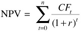
where n = the number of periods; t = the time period; r = the per period cost of capital; and CF t = the cash flow in time period t.
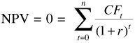
Internal Rate of Return (IRR)
IRR is at present the "truest" rate of return we know how to calculate. Technically, it is the "hurdle" or discount rate that produces an NPV equal to zero. The formula is
A special caution is needed here. The IRR calculation can turn awkward when there is more than one sign change in the cash flow stream. You may get more than one answer for the same series of payments.
One way around the problem is to do a modified IRR in which you calculate the present value of all the outflows ( negatives ) using, say, the company's average interest rate on loans; then compute the IRR using the single outflow figure (CFCM).
The Financial Management Rate of Return (FMRR) developed by Findlay and Messner in 1973 goes one step further. It starts by calculating the present value of all cash outlays, as does the modified IRR, and then calculates a future value for the positive cash flows (inflows). The rate for this future value calculation is the expected rate at which the inflows will be employed.
EAN: 2147483647
Pages: 235