TOLERANCE DESIGN

This section illustrates:

1. How tolerance limits can be set so that the product will meet customer requirements repeatedly with the widest possible tolerances. The goal is to choose the most cost efficient tolerance levels.

2. How prior knowledge about the response characteristics of the component levels of a product can be efficiently used.

DISCUSSION

After the target level for each component has been determined using parameter design, the loss function value of the product design is compared to design guidelines and to the cost of improving the production processes to meet tightened tolerances. If it costs less to tighten the tolerance than the resulting reduction in the loss function, then for the long run it is better to tighten the tolerance. The evaluation of the tolerance limits and the selective tightening of the limits is called tolerance design. As in parameter design, an example will illustrate this approach. The reader may need to review Volume V of this series.

Example

Continuing the example from the previous section, the loss function with low cost tolerance was calculated to be $25.482 per piece or $1,274,100 for the production run of 50,000 pieces. This calculation was based on the assumptions that:

1. The tolerance spread is equal to six times the production standard deviation (C _pk = 1).

2. The response changes linearly across the tolerance limits.

3. The sum of the variance contributions for the components is the total assembly response variance.

4. Humidity was set at levels that are the average humidity ±2 times the standard deviation, and the response changes linearly across these levels.

If any of these assumptions cannot be made, a computer simulation using the appropriate assumptions can be used to determine the total assembly response variance.

The calculation of the response variance was shown in Table 9.58, and we are going to repeat it again. From the response variance contribution table and the calculations, it can be seen that the tolerances for factors A, C, and, to a lesser degree, D are the largest component tolerance contributors to the total response variance. The cost of reducing those tolerances is shown in Table 9.59.

Table 9.59: Cost of Reducing Tolerances

Component	Low Cost Tolerance		High Cost Tolerance		% Reduction	Cost to Change the Tolerance for 50,000 Pieces (dollars)
	Low	High	Low	High
A	-50	+50	-40	+40	20	5,000
C	-5	+5	-4	+4	20	15,000
D	-200	+200	-150	+150	25	9,000

Since the response is linearly related to the component levels, a reduction of 20% in the tolerance spread will result in a reduction of 20% in the response spread. In the situation where the response is not linear, it would be necessary to run a computer simulation, as was mentioned previously.

The impact of tightening the tolerance of each of the three components is summarized in Table 9.60. The variance % reduction per $1000 cost indicates that the reduction of the tolerance of component A should be investigated first since the % reduction per $1000 cost is the greatest.

Table 9.60: The Impact of Tightening the Tolerance

Component	Response Difference Between Tightened Tolerance Limits	Response Production Std. Dev.	Tightened Response Variance	Cost of Tightened Tolerance (dollars)
A	1.76	0.293	0.0858	5000
C	1.76	0.293	0.0858	15,000
D	1.20	0.200	0.0400	9000

Component	Original Variance	Tightened Variance	Variance % Reduction	Variance % Reduction per $1000 Cost
A	0.1344	0.0858	36.16	7.23
C	0.1344	0.0858	36.16	2.41
D	0.0711	0.0400	43.74	4.86

The situation for a reduction of 20% in the tolerance limits of component A is summarized in Table 9.61. The response variance will be 3.9484. If the same 0.5 offset is assumed, the loss function can be calculated as:

Table 9.61: Reduction of 20% in the Tolerance Limits of Component A

Tolerance for Component	Response Difference Between Tol. Limits	Response Production Std. Dev.	Response Variance
A	1.76	0.293	0.0858
B	1.00	0.160	0.0278
C	2.20	0.670	0.1344
D	1.60	0.270	0.0711
E	0.10	0.020	0.0003
			0.3194
Humidity (H)	3.2	0.80	0.6400
Error variance			2.9890
			3.9484

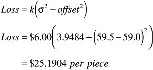
For a production run of 50,000 pieces, the total loss would be $1,259,520. This is a $14,580 decrease in the loss function from the low cost tolerance situation. Since the decrease in the loss function is more than the $5000 cost of tightening the tolerance on A, it is advantageous in the long run to tighten that tolerance.

The 0.50 offset is assumed to be a constant to provide a basis to compare improvement in only the variance part of the equation. In some situations, the actions taken to reduce the response variance may also result in a better-centered response distribution.

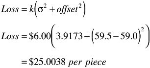
The next step is to evaluate the loss function with the tolerance limits reduced for component D ” see Table 9.62. The response variance will be 3.9173. If the same 0.5 offset is assumed, the loss function can be calculated as:

Table 9.62: Reduction of Tolerance Limits for Component D

Tolerance for Component	Response Difference Between Tol. Limits	Response Production Std. Dev.	Response Variance
A	1.76	0.293	0.0858
B	1.00	0.160	0.0278
C	2.20	0.370	0.1344
D	1.60	0.200	0.0400
E	0.10	0.020	0.0003
			0.2883
Humidity (H)	3.2	0.80	0.6400
Error variance			0.2883
			3.9173

For a production run of 50,000 pieces, the total loss would be $1,250,190. This is a $9330 decrease in the loss function from the situation with only the tolerance of A tightened. Since the decrease in the loss function is more than the $9000 cost of tightening the tolerance on D, it is advantageous in the long run to tighten that tolerance.

We can do the same for component C ” see Table 9.63.

Table 9.63: Reduction of Tolerance Limits for Component C

Tolerance for Component	Response Difference Between Tol. Limits	Response Production Std. Dev.	Respons Variance
A	1.76	0.293	0.0858
B	1.00	0.160	0.0278
C	1.76	0.293	0.0858
D	1.20	0.200	0.0400
E	0.10	0.020	0.0003
			0.2397
Humidity (H)	3.2	0.80	0.6400
Error Variance			2.9890
			3.8687

The response variance will be 3.8687. If the same 0.5 offset is assumed, the loss function can be calculated as:

For a production run of 50,000 pieces, the total loss would be $1,235,610. This is a $14,580 decrease in the loss function from the situation with only the tolerances of A and D tightened. Since the cost of tightening the tolerance on component C is $15,000, it would not be advantageous to tighten that tolerance.

So far, the tolerance design has been entirely a paper exercise based on the tests run during the parameter design and the assumptions about the relationships between the component levels and the response. A set of confirmation runs should be made with the tolerance limits for components A and D tightened. An L8 orthogonal array is used for the confirmation runs with the levels set, test setup, ANOVA table, and level averages as shown in Table 9.64.

Table 9.64: L8 OA used for the Confirmation Runs with the Levels Set, Test Setup, ANOVA Table, and Level Averages

Tolerance Levels
		Low Level	High Level
	Column	(1)	(2)	Nominal
A-Tol.	1	-45	+45	1000
B-Tol.	2	-15	+15	400
C-Tol.	3	-5	+5	60.77
D-Tol.	4	-150	+150	2200
E-Tol.	5	-100	+100	1600
H (Humidity)	6	Low	High	”
Unassigned	7

The test setup and results:

A-Tol	B-Tol	C-Tol	D-Tol	E-Tol	H		Test Result
1	1	1	1	1	1	1	59.7
1	1	1	2	2	2	2	57.5
1	2	2	1	1	2	2	59.5
1	2	2	2	2	1	1	63.6
2	1	2	1	2	1	2	59.3
2	1	2	2	1	2	1	58.6
2	2	1	1	2	2	1	55.8
2	2	1	2	1	1	2	59.3

The average response is 59.2 and the S/N is 28.5. The ANOVA table and level averages for all of the factors from the verification runs are:

ANOVA Table

Source	df	SS	MS	F Ratio	S'	%
A-Tol.	1	6.661	6.661	20.433	6.335	18.35
B-Tol.	1	1.201	1.201	3.684	0.875	2.53
C-Tol.	1	9.461	9.461	29.022	9.135	26.46
D-Tol.	1	2.761	2.761	8.469	2.435	7.05
E-Tol.	1*	0.101	0.101
H	1	13.781	13.781	42.273	13.455	38.98
T	1*	0.551	0.551
Error	”
(pooled error)	2	0.652	0.652		2.282	6.61
Total	7	34.519	4.931

	Level Averages
Factor	Level 1	Level 2
A-Tol	60.1	58.3
B-Tol	58.8	59.6
C-Tol	58.1	60.3
D-Tol	58.6	59.8
E-Tol	59.3	59.1
H	60.5	57.9

As mentioned in the last section, this information cannot be used directly in the loss function since the observed variability may be affected by testing only at the tolerance limits. The center portions of the distributions are not represented in these tests.

Since the change in response is assumed to be a linear increase or decrease across tolerance levels, the loss functions can be easily calculated. The C _pk in production is assumed to be 1.0 or greater for all specified tolerances. The difference between the tolerance limits will be equal to six times the production standard deviation for each component parameter for a C _pk of 1. Since the product response is linearly related to the component parameter level, the difference between the response level averages for the two tolerance limits will equal six times the production response standard deviation. Since the response effect of each component tolerance is additive, the response variance due to each tolerance is additive. In a similar manner, the difference in response between the two humidity levels represents four times the response standard deviation. For this example, the response variance can be calculated as shown in Table 9.65.

Table 9.65: Response Variance

Tolerance for Factor	Response Difference Between Tol. Limits	Response Production Std. Dev.	Variance
A	1.8	0.30	0.0900
B	0.8	0.13	0.0178
C	2.2	0.37	0.1344
D	1.2	0.20	0.0400
E	0.2	0.03	0.001
			0.2833
Humidity (H)	2.6	0.65	0.4225
Error variance			0.3260
			1.0318

The response variance will be 1.0318. The loss function can be calculated from the equation:

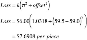
For a production run of 50,000 pieces, the total loss is estimated to be $384,540 compared to $1,274,100 before the tolerance design. This is a $889,560 reduction from the original estimate of the value of the loss function.

The reduction is due to three difference elements:

1. The mean was relocated from 59.5 to 59.2.

2. The error variance was reduced from 2.989 to 0.326.

3. The tolerances for components A and D were tightened.

Humidity

Note that humidity was identified as an important contributor throughout this example. The experimenter should investigate the possibility of controlling humidity to further reduce the loss function. If either the effect of humidity on the design can be minimized or the humidity can be controlled, the loss function could be greatly reduced.

Testing

Eighty tests were used in the example for the last and present sections. These tests were used as follows :

• Determine the target levels ” 64 tests.

• Confirm the choice of targets ” 8 tests.

• Determine the tolerances to tighten ” 0 tests (based on prior knowledge and simulation).

• Confirm the performance with tightened tolerances ” 8 tests.