Section 17.3. Still Images and JPEG Compression

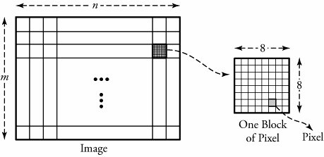
17.3. Still Images and JPEG Compression

This section investigates algorithms that prepare and compress still and moving images. The compression of such data substantially affects the utilization of bandwidths over the multimedia and IP networking infrastructures . We begin with a single visual image, such as a photograph, and then look at video, a motion image. The Joint Photographic Experts Group (JPEG) is the compression standard for still images. It is used for gray-scale and quality- color images. Similar to voice compression, JPEG is a lossy process. An image obtained after the decompression at a receiving end may not be the same as the original.

Figure 17.4 gives an overview of a typical JPEG process, which consists of three processes: discrete cosine transform (DCT), quantization , and compression , or encoding.

Figure 17.4. A typical JPEG process for production and compression of still images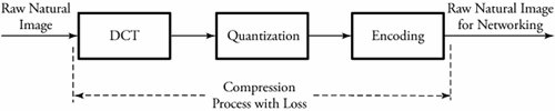

The DCT process is complex and converts a snapshot of a real image into a matrix of corresponding values. The quantization phase converts the values generated by DCT to simple numbers in order to occupy less bandwidth. As usual, all quantizing processes are lossy. The compression process makes the quantized values as compact as possible. The compression phase is normally lossless and uses standard compression techniques. Before describing these three blocks, we need to consider the nature of a digital image.

17.3.1. Raw-Image Sampling and DCT

As with a voice signal, we first need samples of a raw image: a picture . Pictures are of two types: photographs , which contain no digital data, and images , which contain digital data suitable for computer networks. An image is made up of m x n blocks of picture units, or pixels , as shown in Figure 17.5. For FAX transmissions, images are made up of 0s and 1s to represent black and white pixels, respectively. A monochrome image , or black-and-white image , is made up of various shades of gray, and thus each pixel must be able to represent a different shade . Typically, a pixel in a monochrome image consists of 8 bits to represent 2 ⁸ = 256 shades of gray, ranging from white to black, as shown in Figure 17.6.

Figure 17.5. A digital still image

Figure 17.6. Still image in bits: (a) monochrome codes for still image; (b) color codes for still image

JPEG Files

Color images are based on the fact that any color can be represented to the human eye by using a particular combination of the base colors red, green, and blue (RGB). Computer monitor screens, digital camera images, or any other still color images are formed by varying the intensity of the three primary colors at pixel level, resulting in the creation of virtually any corresponding color from the real raw image. Each intensity created on any of the three pixels is represented by 8 bits, as shown in Figure 17.6. The intensities of each 3-unit pixel are adjusted, affecting the value of the 8-bit word to produce the desired color. Thus, each pixel can be represented by using 24 bits, allowing 2 ²⁴ different colors. However, the human eye cannot distinguish all colors among the 2 ²⁴ possible colors. The number of pixels in a typical image varies with the image size .

Example

A JPEG-based computer screen can consist of 1,024 x 1,280 pixels. Consequently, this computer image requires (1,024 x 1,280) x 24 = 31,457,280 bits. If a video consists of 30 images per second, a 943 Mb/s bandwidth is required.

GIF Files

JPEG is designed to work with full-color images up to 2 ²⁴ colors. The graphics interchange format (GIF) is an image file format that reduces the number of colors to 256. This reduction in the number of possible colors is a trade-off between the quality of the image and the transmission bandwidth. GIF stores up to 2 ⁸ = 256 colors in a table and covers the range of colors in an image as closely as possible. Therefore, 8 bits are used to represent a single pixel. GIF uses a variation of Lempel-Ziv encoding (Section 17.6.3) for compression of an image. This technology is used for images whose color detailing is not important, such as cartoons and charts .

DCT Process

The discrete cosine transform (DCT) is a lossy compression process that begins by dividing a raw image into a series of standard N x N pixel blocks. For now, consider a monochrome block of pixels. With a standard size of N = 8, N is the number of pixels per row or column of each block. Let x , y be the position of a particular pixel in a block where 0 x N - 1 and 0 y N - 1. Hence, a gray scale of a given pixel x , y can get an integer value in {0, 1, 2, ..., 255}. For an N x N pixel block, the DCT process is summarized in two steps

1.	Form a P[ x ][ y ] matrix to represent the collection of light-intensity values taken from various points of a real raw image.
2.	Convert the values of P[ x ][ y ]matrix to matrix with normalized and reduced values denoted by T[ i ][ j ] obtained as follows .

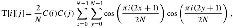
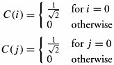
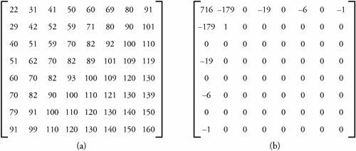
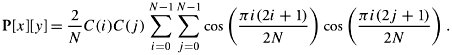
The objective of matrix T[ i ][ j ] is to create as many 0s as possible instead of small numbers in the P[ x ][ y ] matrix in order to reduce the overall bandwidth required to transmit the image. Similarly, matrix T[ i ][ j ] is a two-dimensional array with N rows and N columns , where 0 i N - 1 and 0 j N - 1. The elements of T [ i ][ j ] are known as spatial frequencies and are obtained from

Equation 17.14

where

Example

An 8 x 8 matrix P[ x ][ y ] for an image is formed as shown in Figure 17.7 (a). This matrix is converted to matrix T[ i ][ j ]by using Equation (17.15). This example clearly shows that a matrix as P [ x ][ y ]consisting of 64 values can be converted to T[ i ][ j ] with 9 values and 55 zeros. It is easy to figure out the advantages of this conversion. The 55 zeros can be compressed, conveniently resulting in significant reduction of transmission bandwidth.

Figure 17.7. Matrix examples: (a) P[ x ][ y ]; (b) T[ i ][ j ]

The spatial frequencies depend directly on how much the pixel values change as functions of their positions in a pixel block. Equation (17.15) is set up such that the generated matrix T [ i ][ j ] contains many 0s, and the values of the matrix elements generally become smaller as they get farther away from the upper-left position in the matrix. The values of T [ i ][ j ] elements at the receiver can be converted back to matrix P [ x ][ y ] by using the following function:

Equation 17.15

Note that as values become farther away from the upper-left position, they correspond to a fine detail in the image.

17.3.2. Quantization

To further scale down the values of T[ i ][ j ] with fewer distinct numbers and more consistent patterns to get better bandwidth advantages, this matrix is quantized to another matrix, denoted by Q [ i ][ j ]. To generate this matrix, the elements of matrix T[ i ][ j ] are divided by a standard number and then rounded off to their nearest integer. Dividing T[ i ][ j ] elements by the same constant number results in too much loss. The values of elements on the upper-left portions of the matrix must be preserved as much as possible, because such values correspond to less subtle features of the image. In contrast, values of elements in the lower-right portion correspond to the highest details of an image. To preserve as much information as possible, the elements of T[ i ][ j ]are divided by the elements of an N x N matrix denoted by D[ i ][ j ], in which the values of elements decrease from the upper-left portion to the lower-right portion.

Example.

Consider again the 8 x 8 matrix P[ x ][ y ] already converted to matrix T[ i ][ j ]shown in Figure 17.7. Figure 17.8 (a) shows a divisor matrix D[ i ][ j ]. Figure 17.8 (b) shows the corresponding matrix Q[ i ][ j ] resulting from the quantization process. Note particularly that big values, such as -179 have become smaller and that some such values, as -1 in the upper-right corner turn into 0, making it easier for compression.

Figure 17.8. (a) Divisor matrix D [ i ][ j ] and the quantization of a still image to produce; (b) matrix Q [ i ][ j ] and the order of matrix elements for transmission

We notice here that the process of quantization, as discussed at the beginning of this chapter, is not quite reversible. This means that the values of Q[ i ][ j ] cannot be exactly converted back to T[ i ][ j ], owing mainly to rounding the values after dividing them by D[ i ][ j ]. For this reason, the quantization phase is a lossy process.

17.3.3. Encoding

In the last phase of the JPEG process, encoding finally does the task of compression. In the quantization phase, a matrix with numerous 0s is produced. Consider the example shown in Figure 17.8 (b). The Q matrix in this example has produced 57 zeros from the original raw image. A practical approach to compressing this matrix is to use run-length coding (Section 17.6.1). If run-length coding is used, scanning matrix Q[ i ][ j ] row by row may result in several phrases.

A logical way to scan this matrix is in the order illustrated by the arrows in Figure 17.8 (b). This method is attractive because the larger values in the matrix tend to collect in the upper-left corner of the matrix, and the elements representing larger values tend to be gathered together in that area of the matrix. Thus, we can induce a better rule: Scanning should always start from the upper-left corner element of the matrix. This way, we get much longer runs for each phrase and a much lower number of phrases in the run-length coding.

Once the run-length coding is processed, JPEG uses some type of Huffman coding or arithmetic coding for the nonzero values. Note here that, so far, only a block of 8 x 8 pixels has been processed . An image consists of numerous such blocks. Therefore, the speed of processing and transmission is a factor in the quality of image transfer.