14.5 Multiclass Open Models with LD Devices

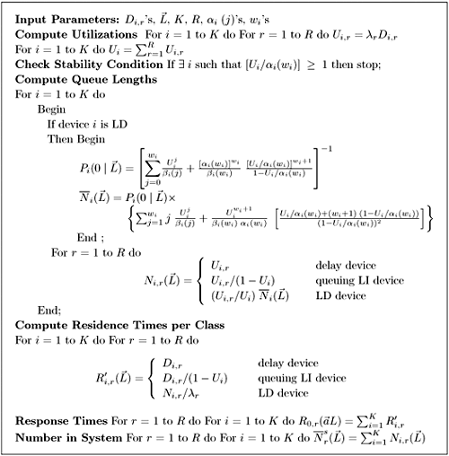
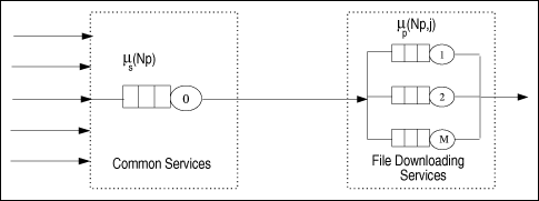
The algorithm presented in this section is an extension of the algorithm presented in Chapter 13 for solving multiple-class open queuing networks. Load-dependent servers are incorporated here. Similar to the closed queuing network case, it is assumed that the service rate-multiplier of any load-dependent device is class independent (i.e., if device i is load-dependent, then a_i,r(j) = a_i(j) for all classes r). As discussed in Chapter 13, the solution to an open queuing network exists only if the stability condition is satisfied. In the case of load-dependent multiclass open networks with class-independent service multipliers, the stability condition is

Equation 14.5.19

If device i is load-independent, a_i(j) = 1 for all j and the stability condition reduces to Let be the vector (l₁, ···, l_R) of arrival rates per class. Let P_i(j | ) be the probability that there are j customers, irrespective of their classes, at device i given that the arrival rate vector is .

The residence time, , of a class r customer at device i is given by

Equation 14.5.20

where R_i,r() is the average response time per visit to device i of a class r customer. This can be computed from Little's result as

Equation 14.5.21

where is the average number of class r jobs at device i and l_i,r is the average arrival rate of class r jobs at device i. It can be proved (see [9]) that

Equation 14.5.22

where is the average total number of customers at device i. can be computed from the device probabilities as

Equation 14.5.23

The probability distribution of node i is given by [9]:

Equation 14.5.24

where b(j) = a(1) x ... x a(j). The probability P_i(0 | ) results from requiring that all probabilities sum to 1. Thus,

Equation 14.5.25

Assuming that the service-rate multipliers become constant after some value w_i, as it is true in most practical cases, closed-form expressions are obtained for the probabilities P_i(j | ) and for . The stability condition in this case becomes a_i(w_i) < 1. Assuming that a_i(j) = a_i(w_i) for j w_i (see Exercise 14.7):

Equation 14.5.26

Equation 14.5.27

and

Equation 14.5.28

The Service Demand Law implies that U_i,r = l_rD_i,r and in the above equations. The result is an algorithm to solve multiclass open queuing networks with load-dependent servers as a function of the class service demands and the class arrival rates. Figure 14.9 displays this algorithm. R_0,r() denotes the average system response time of class r customers and denotes the average number of class r customers in the system.

Figure 14.9. Exact multiclass open QN algorithm with LD devices.

Example 14.5.

Peer-to-peer (P2P) networking is viewed as a new paradigm for constructing distributed applications. In contrast to client-server applications, a peer is both a requester and provider of services. In other words, all peers in a P2P system have the ability to function both as a client and as a server depending on the specific context. Peer-to-peer applications have been used mainly for sharing video, audio files and software. P2P architectures can be classified into three basic categories: centralized service location, distributed service location with flooding, and distributed service location with hashing [7].

In client-server computing, clients generate the workload, which is then processed by the servers. Unlike CS computing, peers generate workloads (e.g., requests for downloading files), but also provide the capacity to process workloads. P2P workloads are examined in detail in [17]. There are many issues surrounding the performance of P2P architectures, such as the impact of the size and characteristics of the user population, the influence of different search strategies, and the consequences of P2P traffic on the underlying networks.

Consider a hypothetical P2P file sharing system, composed of a large number of peers. The system has a centralized service location architecture. To locate a file, a peer sends a query to the central server, which performs a directory lookup and identifies the peers where the files are located. The central server maintain directories of the shared files stored on the peers registered in the system. This service is a common service because it serves all requests. Once the desired file has been located, a peer-to-peer interaction is established to download the file. Assume that the system receives l requests/sec, where a request consists of downloading a file. A QN model is used here to calculate the average time to download a file.

This example presents a simple performance model of a P2P file sharing application based on the modeling technique proposed in [7], which is a novel approach of using QN models to analyze performance. The abstraction presented by the model associates a single server queue with each distinct file in the system. After going through the central server, all requests to download a specific file are required to join the queue associated with the file to be served, as shown in Figure 14.10. The service rate of the server that represents a given file varies with 1) the number of replicas of the file in the P2P application, 2) the popularity of that particular file, and 3) the total load of the system. Thus, the overall queuing model consists of a load-independent server representing the common service component (i.e., the central server) and a set of load-dependent servers, representing the files in the system.

Figure 14.10. Model of a peer-to-peer file sharing system.

The response time of a request is a combination of two factors:

Equation 14.5.29

The common service rate (i.e., the file location service) is independent of the number of peers and is given by:

Equation 14.5.30

where N_p denotes the number of active peers in the system.

Studies indicate that Zipf's Law [21] can be used to characterize the access frequency to Internet objects. Zipf's Law was originally applied to the relationship between a word's popularity in terms of rank and its frequency of use. When one ranks the popularity of events, Zipf's Law states that the size y of the r^th largest occurrence of the event is inversely proportional to its rank. This means that y ~ r^a. It can be shown that

Equation 14.5.31

where p_j is the probability associated with event j, K is a constant and a is the scaling parameter of the distribution. The data shown in [2] indicates that Zipf's Law applies to files serviced by Web servers. This means that the n-th most popular document is exactly twice as likely to be accessed as the 2n-th most popular document, when a = 1, regardless of K.

The service rate for a given file in the system is directly proportional to the number of replicas of that file and to the load of the system (i.e., the number of active peers) [7]. The number of replicas is assumed to be proportional to the popularity of files. Thus, Zipf's Law is used to model the number of replicas providing an estimated download service rate given by:

Equation 14.5.32

where H represents the service rate brought to the system by a single peer (i.e., its contribution to the system's capacity).

Consider a small system with three types of files: software, music, and video. A collection of peers generates the three types of requests to the system. Assume that the P2P system has 30 peers connected by links of 200 Kbps. Let H be 1 download/sec, which corresponds to the time needed to download a 0.2 Mb file, using a 200-Kbps link. Assume that all files are equally popular, implying no file replicas and that K/j^a = 1. Thus, using Eq. (14.5.32) it follows that the file download rate is m_f(N_p) = N_p x H = N_p downloads/sec. However, as has been observed [8], there are two types of peers, freeloaders and non-freeloaders. Freeloaders are those peers that only download files for themselves without providing files to be further downloaded by others. Thus, using this type of evidence, it is assumed that only 10% of the peers (i.e., 3) contribute to the total capacity of the system. This indicates that the service rate multiplier for the file download queue is given by:

Table 14.6 shows the estimated data for each type of request at the central server. The average file download times, using the algorithm in Figure 14.9, are 4.12 sec, 6.85 sec, and 10.94 sec, respectively, for software, music, and video files. The average queue length of the load-dependent device is 12.56 requests.

Table 14.6. Parameterization Data for Example 14.5

Request Type	Avg. Arrival Rate (req./sec)	Mean File Size (Mb)	Server Demands (sec)
			Processor	Disk
Software	1.0	0.18	0.005	0.015
Music	0.6	0.30	0.015	0.012
Video	0.4	0.48	0.010	0.008