Performing a What-If Analysis

What-if analysis is perhaps the most basic method for understanding worksheet data. With what-if analysis, you first calculate a formula D, based on the input from variables A, B, and C. You then say, "What if I change variable A? Or B or C? Or all three? What happens to the result?"

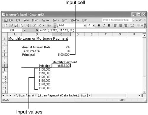
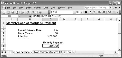
For example, Figure 2.1 shows a worksheet that calculates the monthly payment for a loan or mortgage based on three variables: the interest rate, the term, and the initial principal. Cell C8 shows the result of the PMT() function. Now the questions begin: What if the interest rate is 8%? What if the term is 25 years? What if the principal is $125,000? Or $150,000? Answering these questions is a straightforward matter of changing the appropriate variables and watching the effect on the result.

Figure 2.1. The most basic form of what-if analysis involves changing worksheet variables and watching the result.

More Info

I adapted some of the material in this chapter from my book Formulas and Functions for Microsoft Excel 2003 (Que Publishing, 2004). If you need more detail about data analysis in Excel, you can check out the book at your local store or online at www.mcfedries.com/ExcelFormulas/.

This Chapter's Examples

You'll find the workbook that contains this chapter's examples at www.mcfedries.com/OfficeGurus/.

Performing What-If Analysis with a Range Snapshot

The simplest form of what-if analysis involves changing the value of one cell and watching its effect on the values of one or more other cells. However, what if the cells you want to watch reside in another worksheet or workbook? You could arrange the windows accordingly, but Excel has an easier method: the Camera tool. The Camera takes a snapshot of a specified range and enables you to add that snapshot to any worksheet. The snapshot is "live," however, so any changes that occur in the original range will also appear automatically in the snapshot.

To begin, follow these steps to display the Camera tool:

1.	Select Tools, Customize to display the Customize dialog box.
2.	Select the Commands tab.
3.	In the Categories list, select Tools.
4.	In the Commands list, click and drag the Camera item and drop it on the menu bar.
5.	Click Close.

To use the camera, select the range, click Camera, and then click the spot where you want the snapshot to appear.

Setting Up a One-Input Data Table

Modifying formula variables suffers from a serious drawback: you see only a single result at one time. If you want to study the effect a range of values has on the formula, you need to construct a data table. In the loan payment worksheet, for example, suppose that you want to see the payments with the principal varying between $100,000 and $150,000. You could just enter these values into a row or column and then create the appropriate formulas. Setting up a data table, however, is much easier, as the following procedure shows:

1.	Add to the worksheet the values you want to input into the formula. You have two choices for the placement of these values: If you want to enter the values in a row, start the row one cell up and one cell to the right of the formula. If you want to enter the values in a column, start the column one cell down and one cell to the left of the cell containing the formula, as shown in Figure 2.2. Figure 2.2. To set up the data table, first enter the formula's input values.
2.	Select the range that includes the input values and the formula. (In Figure 2.2, this is B8:C14.)
3.	Choose Data, Table. Excel displays the Table dialog box.
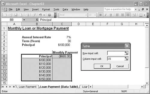
4.	How you fill in this dialog box depends on how you set up your data table: If you entered the input values in a row, use the Row Input Cell text box to enter the cell address of the input cell. If the input values are in a column, enter the input cell's address in the Column Input Cell text box. In the loan payment example, enter C5 (the Principal cell) in the Column Input Cell, as shown in Figure 2.3. Figure 2.3. In the Table dialog box, enter the input cell where you want Excel to substitute the input values.
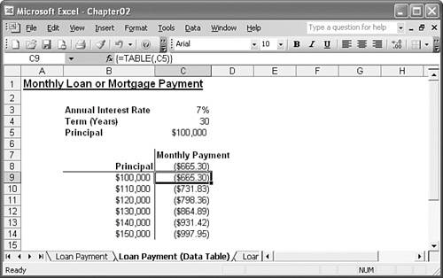
5.	Click OK. Excel places each of the input values in the input cell; Excel then displays the results in the data table, as shown in Figure 2.4. Figure 2.4. Excel substitutes each input value into the input cell and displays the results in the data table.

Setting Up a Two-Input Table

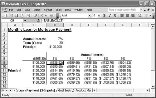
You also can set up data tables that take two input variables. For example, this would enable you to see the effect on a loan payment's value when you enter different values for the principal and the interest rate, for instance. The following steps show you how to set up a two-input data table:

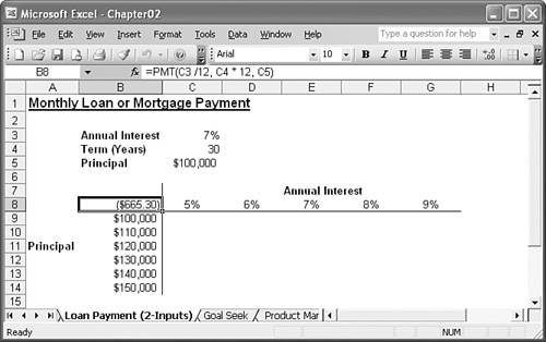
1.	Enter one set of values in a column below the formula and the second set of values to the right of the formula in the same row, as shown in Figure 2.5. Figure 2.5. Enter the two sets of values that you want to input into the formula.
2.	Select the range that includes the input values and the formula (B8:G14 in Figure 2.5).
3.	Choose Data, Table to display the Table dialog box.
4.	In the Row Input Cell text box, enter the cell address of the input cell that corresponds to the row values you entered (C3 in Figure 2.5the Annual Interest variable).
5.	In the Column Input Cell text box, enter the cell address of the input cell you want to use for the column values (C5 in Figure 2.5the Principal variable).
6.	Click OK. Excel runs through the various input combinations and then displays the results in the data table, as shown in Figure 2.6. Figure 2.6. Excel substitutes each input value into the input cell and displays the results in the data table.

Bypassing Table Recalculation

If you make changes to any of the variables in a table formula, Excel recalculates the entire table. This can be a problem with large tables, which can take a long time to calculate. If you prefer to control the table recalculation, choose Tools, Options. Select the Calculation tab and then activate the Automatic Except Tables check box. This tells Excel not to include data tables when it recalculates a worksheet. To recalculate a table, press F9 (or Shift+F9 to recalculate the current worksheet only).

Editing a Data Table

If you want to make changes to the data table, you can edit the formula (or formulas) as well as the input value. However, the data table results are a different matter. When you run the Data, Table command, Excel enters an array formula in the interior of the data table. This formula is a TABLE() function (a special function available only by using the Data, Table command) with the following syntax:

 {=TABLE(row_input_ref, column_input_ref)} 

Here, row_input_ref and column_input_ref are the cell references you entered in the Table dialog box. The braces ({ }) indicate that this is an array, which means that you can't change or delete individual elements of the array. If you want to change the results, you need to select the entire data table and then run the Data, Table command again. If you just want to delete the results, you must first select the entire array and then delete it.