8.2. Sorting and Filtering a Table As you've seen, Excel tables make it easier to enter, edit, and manage large collections of information. Now it's time to meet two of the most useful table features: -
Sorting lets you order the items in your table alphabetically or numerically according to the information in a column. By using the correct criteria, you can make sure the information you're interested in appears at the top of the column, and you can make it easier to find an item anywhere in your table. -
Filtering lets you display only certain records in your table based on specific criteria you enter. Filtering lets you work with part of your data and temporarily hide the information you aren't interested in. You can quickly apply sorting and filtering using the drop-down column headers that Excel adds to every table.
Note: Don't see a drop-down list at the top of your columns ? A wrong ribbon click can inadvertently hide them. If you just see ordinary column headings (and you know you have a bona fide table), choose Data  Sort & Filter Filter to get the drop-down lists back. Sort & Filter Filter to get the drop-down lists back.
8.2.1. Applying a Simple Sort Order Before you can sort your data, you need to choose a sorting key the piece of information Excel uses to order your records. For example, if you want to sort a table of products so the cheapest (or most expensive) products appear at the top of the table, the Price column would be the sorting key to use. In addition to choosing a sorting key, you also need to decide whether you want to use ascending or descending order. Ascending order, which is most common, organizes numbers from smallest to largest, dates from oldest to most recent, and text in alphabetical order. (If you have more than one type of data in the same columnwhich is rarely a good ideatext appears first, followed by numbers and dates, then true or false values, and finally error values.) In descending order, the order is reversed . To apply a new sort order, choose the column you want to use for your sort key. Click the drop-down box at the right side of the column header, and then choose one of the menu commands that starts with the word "Sort." The exact wording depends on the type of data in the column, as follows : -
If your column contains numbers , you see "Sort Smallest to Largest" and "Sort Largest to Smallest". -
If your column contains text , you see "Sort A to Z" and "Sort Z to A" (see Figure 8-8). -
If your column contains dates , you see "Sort Oldest to Newest" and "Sort Newest to Oldest". When you choose an option, Excel immediately reorders the records, and then places a tiny arrow in the column header to indicate that you used this column for your sort. However, Excel doesn't keep re-sorting your data when you make changes or add new records (after all, it would be pretty distracting to have your records jump around unexpectedly). If you make some changes and want to reapply the sort, just go to the column header menu and choose the same sort option again. If you click a second column, and then choose Sort Ascending or Sort Descending, the new sort order replaces your previous sort order. In other words, the column headers let you sort your records quickly, but you can't sort by more than one column at a time.  | Figure 8-8. A single click is all it takes to order records in ascending order by their category names . You don't need to take any action to create these handy drop-down listsExcel automatically provides them for every table. | |
8.2.2. Sorting with Multiple Criteria Simple table sorting runs into trouble when you have duplicate values. Take the product table sorted by category in Figure 8-8, for example. All the products in the Communications category appear first, followed by products in the Deception category, and so on. However, Excel doesn't make any effort to sort products that are in the same category. For example, if you have a bunch of products in the Communications category, then they appear in whatever order they were in on your worksheet, which may not be what you want. In this case, you're better off using multiple sort criteria . With multiple sort criteria, Excel orders the table using more than one sorting key. The second sorting key springs into action only if there are duplicate values in the first sorting key. For example, if you sort by Category and Model Name, Excel first separates the records into alphabetically ordered category groups. It then sorts the products in each category in order of their model name . To use multiple sort criteria, follow these steps: -
Move to any one of the cells inside your table, and then choose Home Editing Sort & Filter Custom Sort . Excel selects all the data in your table, and then displays the Sort dialog box (see Figure 8-9) where you can specify the sorting keys you want to use. 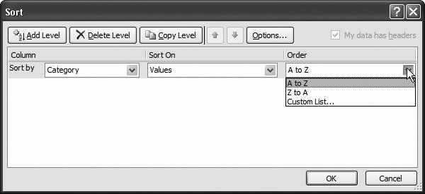 | Figure 8-9. To define a sorting key, you need to fill in the column you want to use (in this example, Category). Next , pick the information you want to use from that column, which is almost always the actual cell values (Values). Finally, choose the order for arranging values, which depends on the type of data. For text values, as in this example, you can pick A to Z, Z to A, or Custom List (Section 2.2.3.1). | |
Note: You can use the Home Editing Sort & Filter Custom Sort command with any row-based data, including information thats not in a table. When you use it with non-table data, Excel automatically selects the range of cells it believes constitutes your table.
-
Fill in the information for the first sort key in the Column, Sort On, and Order columns . Figure 8-9 shows how it works. -
If you want to add another level of sorting, click Add Level, and then follow the instructions in step 2 to configure it . You can repeat this step to add as many sorting levels as you want (Figure 8-10). Remember, it makes sense to add more levels of sorting only if there's a possibility of duplicate value in the levels you've added so far. For example, if you've sorted a bunch of names by last name, you want to sort by first name, because some people may share the same last name. However, it's probably not worth it to add a third sort on the middle initial, because very few people share the same first and last name. 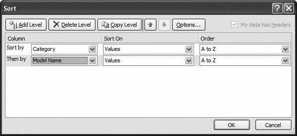 | Figure 8-10. This example shows two sorting keys: the Category column and the Model Name column. The Category column may contain duplicate entries, which Excel sorts in turn according to the text in the Model Name column. When you're adding multiple sort keys, make sure they're in the right order. If you need to rearrange your sorting, select a sort key, and then click the arrow buttons to move it up the list (so it's applied first) or down the list (so it's applied later). | | -
Optionally, click the Options button to configure a few finer points about how your data is sorted . For example, you can turn on case-sensitive sorting, which is ordinarily switched off. If you switch it on, travel appears before Travel . -
Click OK . Excel sorts your entire table based on the criteria you've so carefully specified (Figure 8-11).  | Figure 8-11. The worksheet shows the following sort's result: alphabetically ordered categories, each of which contains a subgroup of products that are themselves in alphabetical order. | |
8.2.3. Filtering with the List of Values Sorting is great for ordering your data, but it may not be enough to tame large piles of data. You can try another useful technique, filtering , which lets you limit the table so it displays only the data that you want to see. Filtering may seem like a small convenience, but if your table contains hundreds or thousands of rows, filtering is vital for your day-to-day worksheet sanity . Here are some situations where filtering becomes especially useful: -
To pluck out important information, like the number of accounts that currently have a balance due. Filtering lets you see just the information you need, saving you hours of headaches . -
To print a report that shows only the customers who live in a specific city. -
To calculate information like sums and averages for products in a specific group . POWER USERS' CLINIC
Sorting with a Custom List | | Most of the time, you'll want to stick with the standard sorting orders. For example, you'll put numbers in numeric order, dates in chronological order, and text in alphabetical order. But not always. For example, you may have good reason to arrange the categories in Figure 8-11 in a different order that puts more important categories at the top of the table. Or, you may have text values that have special meaning and are almost always used in a specific non-alphabetical order, like the days of the week (Sunday, Monday, Tuesday, and so on) or calendar months (January, February, March, April, and so on). You can deal with these scenarios with a custom list that specifies your sort order. In the Order column, choose Custom List. This choice opens the Custom List dialog box, where you can choose an existing list or create a new one by selecting NEW LIST and typing in your values. (Section 2.2.3.1 has more on creating specialized lists.) Figure 8-12 shows an example. Custom list sorting works best when you have a relatively small number of values that never change. If you have dozens of different values, it's probably too tedious to type them all into a custom list. |
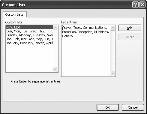 | Figure 8-12. Using a custom list for your sort order, you can arrange your categories so that Travel always appears at the top, as shown here. Once you've finished entering a custom list, click Add to store the list for future use. | |
Automatic filtering, like sorting, uses the drop-down column headings. When you click the drop-down arrow, Excel shows a list of all the distinct values in that column. Figures 8-13 and 8-14 show how filtering works on the Category column. 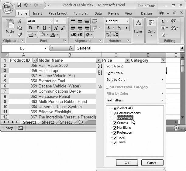 | Figure 8-13. Initially, each value has a checkmark next to it. Clear the checkmark to hide rows with that value. (In this example, products in the Deception category won't appear in the table.) Or, if you want to home in on just a few items, clear the Select All checkmark to remove all the checkmarks, and then choose just the ones you want to see in your table, as shown in Figure 8-14. | |
To remove a filter, open the drop-down column menu, and choose Clear Filter. 8.2.4. Creating Smarter Filters The drop-down column lists give you an easy way to filter out specific rows. However, in many situations you'll want a little more intelligence in your filtering. For example, imagine you're filtering a list of products to focus on all those that top $100. You could scroll through the list of values, and remove the checkmark next to every price that's lower than $100. What a pain in the neck that would be. 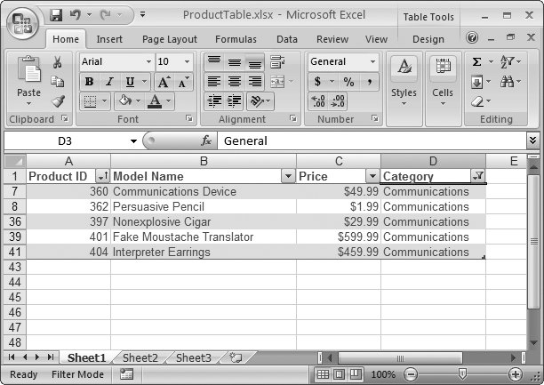 | Figure 8-14. If you select Communications and nothing else from the Category list in the product table example, the table displays only the five products in the Communications category. | |
Thankfully, Excel has more filtering features that can really help you out here. Based on the type of data in your column (text, a number, or date values), Excel adds a wide range of useful filter options to the drop-down column lists. You'll see how this all works in the following sections. 8.2.4.1. Filtering dates You can filter dates that fall before or after another date, or you can use preset periods like last week, last month, next month, year-to-date, and so on. To use date filtering, open the drop-down column list, and choose Date Filters. Figure 8-15 shows what you see. 8.2.4.2. Filtering numbers For numbers, you can filter values that match exactly, numbers that are smaller or larger than a specified number, or numbers that are above or below average. 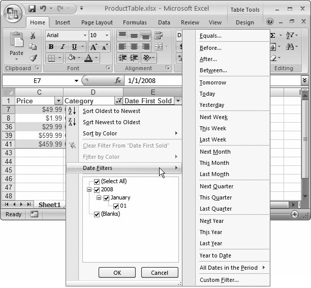 | Figure 8-15. Shown here is the mind-boggling array of ready-made date filtering options you can apply to a column that contains dates. For example, choose Last Week to see just those dates that fall in the period Sunday to Saturday in the previous week. | |
To use number filtering, open the drop-down column list, choose Number Filters, and then pick one of the filter options. For example, imagine you're trying to limit the product list to show expensive products. You can accomplish this quite quickly with a number filter. Just open the drop-down column list for the Price column, and then choose Number Filters Greater Than Or Equal To. A dialog box appears where you can supply the $100 minimum (Figure 8-16). 8.2.4.3. Filtering text For text, you can filter values that match exactly, or values that contain a piece of text. To apply text filtering, open the drop-down column list, and then choose Text Filters. 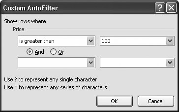 | Figure 8-16. This dialog box lets you complete the Greater Than Or Equal To filter. It matches all products that are $100 or more. You can use the bottom portion of the window (left blank in this example) to supply a second filter condition that either further restricts (choose And) or supplements your matches (choose Or). | |
WORKAROUND WORKSHOP
The Disappearing Cells | | Table filtering's got one quirk. When you filter a table, Excel hides the rows that contain the filtered records. In fact, all Excel really does is shrink each of these rows to have a height of 0 so they're neatly out of sight. The problem? When Excel hides a row, it hides all the data in that row, even if the data is not a part of the table . That property means that if you place a formula in one of the cells to the right of the table, then this formula may disappear from your worksheet temporarily when you filter the table! This behavior is quite a bit different from what happens if you delete a row, in which case cells outside the table aren't affected. If you frequently use filtering, you may want to circumvent this problem by putting your formulas underneath or above the table. Generally, putting the formulas above the table is the most convenient choice because the cells don't move as the table expands or contracts. |
If you're performing filtering with text fields, you can gain even more precise control using wildcards. The asterisk (*) matches any series of characters , while the question mark (?) matches a single character. So the filter expression Category equals T* matches any category that starts with the letter T. The filter expression Category equals T???? matches any five-letter category that starts with T. |