4.6 Data Sources and Sinks

4.6 Data Sources and Sinks

Data sources and sinks are tools to provide directionality to flows. A data source generates a traffic flow, and a data sink terminates a traffic flow. To help show data sources and sinks in a diagram, the convention shown in Figure 4.15 is used. Data sources are represented as a circle with a dot in the center, and a data sink is represented as a circle with a cross (i.e., star or asterisk) in the center. These are 2D representations of a plane with an arrow coming out of it, as in traffic flowing out of a source, or a plane with an arrow going into it, as in traffic flowing into a sink. By using these symbols, we can show data sources and sinks on a 2D map without the need for arrows.

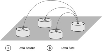
Figure 4.15: Convention for data sources and sinks.

Almost all devices on a network will produce and accept data, acting as both data sources and data sinks, although some device will typically act as either a source or a sink. In addition, a device may be primarily a data source or sink for a particular application.

Some examples of data sources are devices that do a lot of computing or processing and generate large amounts of information, such as computing servers, mainframes, parallel systems, or computing clusters. Other (specialized) devices, such as cameras, video production equipment, application servers, and medical instruments, do not necessarily do a lot of computing (in the traditional sense) but can still generate a lot of data, video, and audio that will be transmitted on the network (Figure 4.16).

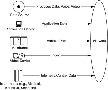
Figure 4.16: Example data sources.

A good example of a data sink is a data-storage or archival device. This may be a single device, acting as a front end for groups of disk or tape devices. Devices that manipulate or display large quantities of information, such as video-editing or display devices, also act as data sinks (Figure 4.17).

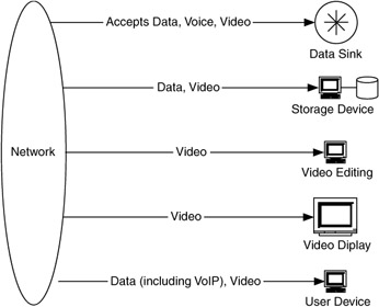
Figure 4.17: Example data sinks.

Example 4.2: Data Sources and Sinks for Data Migration Applications.

As an example, let's consider the data-migration applications. Recall that Figure 4.8 shows device location information for these applications. Shown on this map are storage and compute servers, a video source, and groups of desktop devices for each building. Note that a total number of desktop devices is given, simplifying the map and flows. If more detail is needed, this group could be separated into multiple groups, based on their requirements, or single devices can be separated. If necessary, a new map could be generated for just that building, with substantially more detail.

This service has two applications. Application 1 is the frequent migration of data on users' desktops, servers, and other devices to storage servers at each campus. As part of this application, data are migrated from the server at the central campus to the server at the north campus.

The server at the south campus is also the archival (or long-term) server for these campuses. Application 2 is the migration of data that have been collected over a specific period (e.g., 1 day) from the server at the central campus to the archival server at the south campus.

When we add the data sources and sinks for Application 1 to Figure 4.13, we get Figure 4.18, in which all devices are labeled as a data source, a data sink, or both. All of the user devices at each campus are data sources. The servers at the central campus act as a data sink for flows from user devices at that campus and as a data source when data migrate to the server at the north campus (flow F4). The server at the south campus is a data sink for user flows at that campus, and the servers at the north campus are data sinks for all devices at that campus, including servers and digital video, as well as for flow F4 from the central campus.

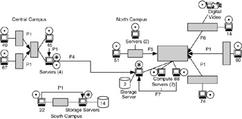
Figure 4.18: Data sources, sinks, and flows added to first part of Application 1.

With the sources and sinks on the map, along with arrows between them to indicate potential traffic flows, we are beginning to have an idea of where flows are occurring in this network for this application.

We do the same thing to Application 2, with the result shown in Figure 4.19. For this part of the application, the desktop devices and video source are not involved, so they are not shown as either sources or sinks of data. The server at the central campus that was a data sink for Application 1 now becomes a data source for Application 2, sending data to the archival server (shown as a data sink). The flows for this part of the application are much simpler, merely a single flow between the storage server and the archival device. This is shown in two ways: as a flow between buildings (option 1, the standard convention used so far in this example) and as a flow between devices at separate buildings (option 2). Although option 2 is not common practice, it is used here because there are only two devices (and one flow) for this application.

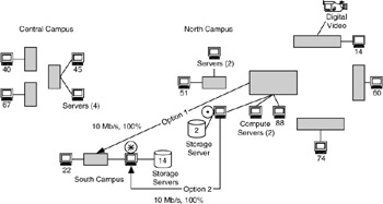
Figure 4.19: Data sources, sinks, and flows added to Application 2 (two options shown).

These applications are shown as separate events to clarify the flows and the roles of the storage servers. We could, however, put both parts of the application together on the same map. We would want to ensure that the resultant map is still clear about when devices are data sources and sinks.

One way to simplify this map is to focus on only flows between storage servers, data sources, and sinks. Figure 4.20 shows this case, with both applications on the same map.

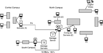
Figure 4.20: Data-migration application with server-server flows isolated.

You may have noticed in the previous example that flows occur at different times of the day and can vary in schedule (when they occur), frequency (how often they occur), and duration (how long they last). The occurrence of traffic flows can be cyclic (e.g., every Monday morning before 10 AM, at the end of each month, and during the end-of-the-year closeout). Understanding when flows occur and how they affect your customer's business or operation is critical. For example, if 90% of the revenue for a business is generated the last 4 weeks before Christmas, you may need to focus flow development on what is happening to applications during that time.

This leads to the concept of developing worst-case and typical-usage scenarios. This is similar to developing for single-tier or multitier performance, as discussed in Chapter 3. Worst-case scenarios are like those described earlier for a business whose revenue is highly seasonal. This is similar to developing for the highest-performance applications and devices in that your focus is on times when the network requires its greatest performance to support the work being done. Architecting/designing a network for the worst-case scenario can be expensive and will result in overengineering the network for most of its life cycle. Therefore, the customer must be fully aware and supportive of the reasons for building toward a worst-case scenario.

Typical-usage scenarios describe an average (typical) workload for the network. This is similar to developing for single-tier performance in that your focus is on times when average, everyday work is being done. Recall from Chapter 3 that single-tier performance focuses on those applications and devices that are in general use and that make up a background level of traffic on the network. This is the average everyday work that forms a typical-usage scenario. Often both worst-case and typical-usage scenarios are developed for a network.

Using data sources and sinks to help map flows for an application provides a great start to generating the flows for your network. Flow models, described next, is another great tool that you can use to help describe flows.