Right Idea, Wrong Distribution

For this purpose, my dear friend and colleague, Pascal Leroy^[4], suggested the skewed lognormal distribution^[5], which more accurately reflects many phenomena in nature.

^[4] No relation to Roscoe! Pascal is a real person living in France, who has often improved the quality of my writing through insightful criticism.

^[5] The lognormal is actually a "family" of distributions, of which we have chosen just one. For more information on the ubiquity of the lognormal distribution, see LogNormal Distributions Across the Sciences: Keys and Clues, Eckhard Limpert, Werner A. Stahl, and Markus Abbt, BioScience May 2001, Vol. 51, No. 5, page 341.

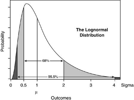
Unlike the standard normal distribution, the lognormal distribution is asymmetrical and lacks a left tail that stretches to infinity. Figure 9.5 shows what it looks like.

Figure 9.5. The lognormal distribution for depicting positive outcomes only.

We still use a sigma to represent the standard deviation, but we interpret it differently for the lognormal distribution, as explained next. Note that µ is now coincident with 1 sigma. Half the area under the curve is to the left of 1 sigma and half is to the right; if we believe the universe of projects has this distribution, then we want our project to fall to the right of the 1 sigma line, which means its reward will be above the average.^[6] This is the equivalent of saying that we are willing to invest µ (or 1 sigma) to do the project; any outcome (payoff, reward) less than that represents a loss (red ink), and anything above that is a win. To put it another way, we have "shifted" the lognormal distribution such that µ (s = 1) corresponds to breakeven or zero net payoff.

^[6] Actually, the math is a little more complicated than that. For the standard normal distribution, the mean and the median are identical because of the symmetry of the distribution. For the lognormal distribution, they are not. So taking the 1 sigma point here is a little off, but the effect is small. We will ignore it in all that follows, as the effect is on the order of a few percent, and our overall model is not that precise anyway.

Unlike the standard normal distribution, the lognormal distribution clumps unsuccessful projects between zero and 1 sigma, and successful projects range from 1 sigma to infinity with a long, slowly diminishing tail. This tells us that we have a small number of projects with very large payoffs to the right, but our losses are limited on the left. This seems to be a better model of reality.

The meaning of sigma is different in this distribution. As you move away from the midpoint, which is labeled here as 1 sigma, you accrue area a little differently. Each confidence interval corresponds to a distance out to ((1/2)ⁿ x sigma) on the left, and out to (2ⁿ x sigma) on the right. This means that 68 percent of the area lies between 0.5 sigma and 2 sigma, and 95.5 percent of the area lies between 0.25 sigma and 4 sigma. This is how the multiplicative nature of the lognormal distribution manifests itself.

Mathematically, the distribution results from phenomena that statistically obey the multiplicative central limit theorem. This theorem demonstrates how the lognormal distribution arises from many small multiplicative random effects. In our case, one could argue that all variance in the outcomes of software development projects is due to many small but multiplicative random effects. By way of contrast, the standard normal distribution results from the additive contribution of many small random effects.