6.4 Constructing the Interpolation Function
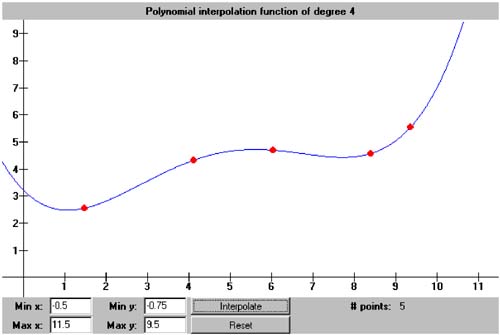
6.4 Constructing the Interpolation Function From the equations for the b i coefficients in the previous section, we see that they are values at the top of each column of the divided difference table, starting with the column labeled f ( x ) in Table 6-1. We start with the small DataPoint class in package numbercruncher.mathutils that represents a data point constructed from an x value and a y value. See Listing 6-0. Listing 6-0 A data point. package numbercruncher.mathutils; /** * A data point for interpolation and regression. */ public class DataPoint { /** the x value */ public float x; /** the y value */ public float y; /** * Constructor. * @param x the x value * @param y the y value */ public DataPoint(float x, float y) { this.x = x; this.y = y; } } The InterpolationPolynomial class in package numbercruncher.mathutils represents a polynomial interpolation function in Newton form. It uses divided differences to compute the coefficients. See Listing 6-1a. The class builds the divided difference table incrementally?aeach new data point allows a new entry to be appended at the bottom of each column. Method addDataPoint() augments the table with each new data point. The class implements the Evaluatable interface described at the beginning of Chapter 5. Method at() returns the value of the interpolation function at a given value of x by computing the terms of the Newton form. Listing 6-1a A class that implements a polynomial interpolation function. package numbercruncher.mathutils; /** * A polynomial interpolation function. */ public class InterpolationPolynomial implements Evaluatable { /** number of data points */ private int n; /** array of data points */ private DataPoint data[]; /** divided difference table */ private float dd[][]; /** * Constructor. * @param data the array of data points */ public InterpolationPolynomial(DataPoint data[]) { this.data = data; this.dd = new float[data.length] [data.length]; for (int i = 0; i < data.length; ++i) { addDataPoint(data[i]); } } /** * Constructor. * @param maxPoints the maximum number of data points */ public InterpolationPolynomial(int maxPoints) { this.data = new DataPoint[maxPoints]; this.dd = new float[data.length][data.length]; } /** * Return the data points. * @return the array of data points */ public DataPoint[] getDataPoints() { return data; } /** * Return the divided difference table. * @return the table */ public float[][] getDividedDifferenceTable() { return dd; } /** * Return the current number of data points. * @return the count */ public int getDataPointCount() { return n; } /** * Add new data point: Augment the divided difference table * by appending a new entry at the bottom of each column. * @param dataPoint the new data point */ public void addDataPoint(DataPoint dataPoint) { if (n >= data.length) return; data[n] = dataPoint; dd[n][0] = dataPoint.y; ++n; for (int order = 1; order < n; ++order) { int bottom = n - order - 1; float numerator = dd[bottom+1][order-1] - dd[bottom][order-1]; float denominator = data[bottom + order].x - data[bottom].x; dd[bottom][order] = numerator/denominator; } } /** * Return the value of the polynomial * interpolation function at x. * (Implementation of Evaluatable.) * @param x the value of x * @return the value of the function at x */ public float at(float x) { if (n < 2) return Float.NaN; float y = dd[0][0]; float xFactor = 1; // Compute the value of the function. for (int order = 1; order < n; ++order) { xFactor = xFactor*(x - data[order-1].x); y = y + xFactor*dd[0][order]; } return y; } /** * Reset. */ public void reset() { n = 0; } } Program 6 §C1 instantiates an InterpolationPolynomial object. As shown in Listing 6-1b, the noninteractive version of the program constructs the interpolation function from a set of five data points from e x in the interval 1 < x < 2 as computed by Math.exp() . With each new data point, the interpolation function can estimate the value e 1.4 with greater accuracy. Note that the data points are not sorted, and they are not evenly spaced . Listing 6-1b The noninteractive version of Program 6 §C1 estimates e 1.4 with increasing accuracy as new data points are added to the polynomial interpolation function. package numbercruncher.program6_1; import numbercruncher.mathutils.DataPoint; import numbercruncher.mathutils.InterpolationPolynomial; import numbercruncher.mathutils.AlignRight; /** * PROGRAM 6C1: Polynomial Interpolation * * Demonstrate polynomial interpolation by using a divided difference * table to construct an interpolation function for a set of data points. * Use the function to estimate new values. */ public class Interpolation { private static final int MAX_POINTS = 10; private static AlignRight ar = new AlignRight(); /** * Main program. * @param args the array of runtime arguments */ public static void main(String args[]) { InterpolationPolynomial p = new InterpolationPolynomial(MAX_POINTS); float x = 1.4f; p.addDataPoint(new DataPoint(1.12f, (float) Math.exp(1.12f))); p.addDataPoint(new DataPoint(1.55f, (float) Math.exp(1.55f))); printEstimate(p, x); p.addDataPoint(new DataPoint(1.25f, (float) Math.exp(1.25f))); printEstimate(p, x); p.addDataPoint(new DataPoint(1.92f, (float) Math.exp(1.92f))); printEstimate(p, x); p.addDataPoint(new DataPoint(1.33f, (float) Math.exp(1.33f))); printEstimate(p, x); p.addDataPoint(new DataPoint(1.75f, (float) Math.exp(1.75f))); printEstimate(p, x); } /** * Print the value of p(x). * @param p the polynomial interpolation function * @param x the value of x */ private static void printEstimate(InterpolationPolynomial p, float x) { printTable(p); float est = p.at(x); float exp = (float) Math.exp(x); float errorPct = (float) Math.abs(100*(est - exp)/exp); System.out.println("\nEstimate e^" + x + " = " + est); System.out.println(" Math.exp(" + x + ") = " + exp); System.out.println(" % error = " + errorPct + "\n"); } /** * Print the divided difference table. */ private static void printTable(InterpolationPolynomial p) { int n = p.getDataPointCount(); DataPoint data[] = p.getDataPoints(); float dd[][] = p.getDividedDifferenceTable(); ar.print("i", 1); ar.print("x", 5); ar.print("f(x)", 10); if (n > 1) ar.print("First", 10); if (n > 2) ar.print("Second", 10); if (n > 3) ar.print("Third", 12); if (n > 4) ar.print("Fourth", 12); if (n > 5) ar.print("Fifth", 12); ar.underline(); for (int i = 0; i < n; ++i) { ar.print(i, 1); ar.print(data[i].x, 5); ar.print(dd[i][0], 10); for (int order = 1; order < n-i; ++order) { ar.print(dd[i][order], (order < 3) ? 10 : 12); } ar.println(); } } } Output: i x f(x) First -------------------------- 0 1.12 3.0648541 3.82934 1 1.55 4.71147 Estimate e^1.4 = 4.137069 Math.exp(1.4) = 4.0552 % error = 2.0188677 i x f(x) First Second ------------------------------------ 0 1.12 3.0648541 3.82934 1.8545004 1 1.55 4.71147 4.070425 2 1.25 3.4903429 Estimate e^1.4 = 4.0591803 Math.exp(1.4) = 4.0552 % error = 0.09814953 i x f(x) First Second Third ------------------------------------------------ 0 1.12 3.0648541 3.82934 1.8545004 0.724587 1 1.55 4.71147 4.070425 2.43417 2 1.25 3.4903429 4.971068 3 1.92 6.820958 Estimate e^1.4 = 4.0546155 Math.exp(1.4) = 4.0552 % error = 0.014416116 i x f(x) First Second Third Fourth ------------------------------------------------------------ 0 1.12 3.0648541 3.82934 1.8545004 0.724587 0.17594407 1 1.55 4.71147 4.070425 2.43417 0.7615353 2 1.25 3.4903429 4.971068 2.2666323 3 1.92 6.820958 5.1523986 4 1.33 3.7810435 Estimate e^1.4 = 4.055192 Math.exp(1.4) = 4.0552 % error = 1.998972E-4 i x f(x) First Second Third Fourth Fifth ------------------------------------------------------------------------ 0 1.12 3.0648541 3.82934 1.8545004 0.724587 0.17594407 0.037198737 1 1.55 4.71147 4.070425 2.43417 0.7615353 0.19937928 2 1.25 3.4903429 4.971068 2.2666323 0.80141115 3 1.92 6.820958 5.1523986 2.667338 4 1.33 3.7810435 4.6989512 5 1.75 5.754603 Estimate e^1.4 = 4.0552006 Math.exp(1.4) = 4.0552 % error = 1.1758659E-5 It is often the case, however, that the given set of data points will not come from any known function. Or the function is so expensive to compute that using an interpolation function is preferable. The interactive version [2] of Program 6 §C1 allows you to set up to 10 arbitrary data points by clicking the mouse on the graph, and the program will then create and plot the polynomial interpolation function through the data points. Screen 6-1a shows a screen shot with 5 data points.
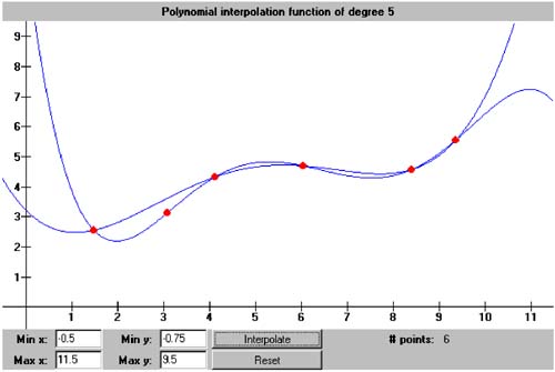
Screen 6-1a. A graph of a polynomial interpolation function created by the interactive version of Program 6 §C1. Screen 6-1b shows the plot of the modified interpolation function after adding a new data point. Screen 6-1b. The result of adding another data point (the second one from the left). With an interpolation function, it is important that we use it to interpolate , not extrapolate. Attempting to use the function to estimate values outside of the domain of the original data values can be very precarious. Screens 6-1a and 6-1b show how the function can shoot off in the positive or negative y directions with x values less than or greater than the original data points. This is especially true with higher degree functions. |

| |
| Top |
EAN: 2147483647
Pages: 141