12.1 Modeling Timed Systems

12.1 Modeling Timed Systems

In Chapter 3, we stated that our model of concurrent execution was asynchronous; processes proceed at arbitrary relative speeds. Consequently, the delay between two successive actions of a process can take an arbitrarily long time. How then do we make processes aware of the passage of time and, in particular, how can we synchronize their execution with time? The answer is to adopt a discrete model of time in which the passage of time is signaled by successive ticks of a clock. Processes become aware of the passage of time by sharing a global tick action. Time is measured as a positive integer value. To illustrate the use of this model of time, we return to the double-click program described in the introduction to the chapter. Figure 12.1 depicts the relationship between discrete time and mouse clicks.

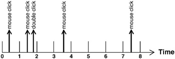
Figure 12.1: Discrete time and mouse clicks.

To make the discussion concrete, assume that the unit of time represented in Figure 12.1 is a second. We specify that a double-click should be recognized when the time between two successive mouse clicks is less than, say, three seconds. We can easily see that the click during period 0 and the click during period 1 constitute a double-click since the interval between these clicks must be less than two seconds. The click during period 3 and the click during period 7 do not form a double-click since there is an interval between these clicks of at least three seconds. The use of discrete time means that we cannot determine precisely when an event occurs, we can only say that it occurs within some period delimited by two ticks of the clock. This gives rise to some timing uncertainty. For example, if the last mouse click happened in period 6, would a double-click have occurred or not? The most we could say is that the last two mouse clicks were separated by at least two seconds and not more than four seconds. We can increase the accuracy by having more ticks per second, however some uncertainty remains. For example, with two ticks per second, we could say that two clicks were separated by at least 2.5 seconds and not more than 3.5 seconds. In fact, this uncertainty also exists in implementations since time is measured in computer systems using a clock that ticks with a fixed periodicity, usually in the order of milliseconds. An implementation can only detect that two events are separated by time (n ± 1) * T, where T is the periodicity of the clock and n the number of clock ticks between the two events. In general, despite the limitations we have discussed above, discrete time is sufficient to model many timed systems since it is also the way time is represented in implementations.

In the example above, if we want to ensure that the clicks which form a double-click are never more than three seconds apart, the last click would have to happen in period 5. Consequently, after the first mouse click occurs, the clock must not tick more than two times before the second click of a double-click occurs. To capture the behavior of the double-click program as a model in FSP, we use the tick action to signal the beginning (and end) of each period. A doubleclick action occurs if less than three tick actions occur between successive mouse clicks. The behavior of the double-click program is modeled as follows:

 DOUBLECLICK(D=3) =   (tick -> DOUBLECLICK | click -> PERIOD[1]), PERIOD[t:1..D] =   (when (t==D) tick -> DOUBLECLICK   |when (t<D)   tick -> PERIOD[t+1]   |click -> doubleclick -> DOUBLECLICK   ).

The DOUBLECLICK process accepts a click action at any time, since, initially, there is a choice between click and tick. When a click occurs, the process starts counting the tick s that follow. If a click occurs before the third succeeding tick, then a doubleclick action is output, otherwise the process resets. Figure 12.2 shows the LTS for DOUBLECLICK and two possible traces of the model; in (a) a doubleclick is output after two clicks and in (b) it is not.

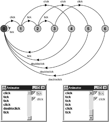
Figure 12.2: DOUBLECLICK LTS and traces.

In discussing the double-click program, we assumed that clock ticks occur every second. However, this is simply an interpretation of the model. We choose an interpretation for a tick that is appropriate to the problem at hand. For example, in modeling hardware circuits, ticks would delimit periods measured in nanoseconds. However, within a particular time frame, the more accurately we represent time, the larger the model. For example, if we wanted to increase the accuracy of the double-click model while retaining the same time frame, we could decide to have two ticks per second and, consequently, the parameter D would become 6 rather than 3. This would double the number of states in DOUBLECLICK.

12.1.1 Timing Consistency

The previous example dealt with how a process is made aware of the passage of time. We now examine the implications of time in models with multiple processes. We look at a simple producer – consumer system in which the PRODUCER process produces an item every Tp seconds and the CONSUMER process takes Tc seconds to consume an item. The models for the PRODUCER and CONSUMER processes are listed below:

 CONSUMER(Tc=3) =   (item -> DELAY[1] | tick -> CONSUMER), DELAY[t:1..Tc] =   (when(t==Tc) tick -> CONSUMER   |when(t<Tc)  tick -> DELAY[t+1]   ). PRODUCER(Tp=3) =   (item -> DELAY[1]), DELAY[t:1..Tp] =   (when(t==Tp) tick -> PRODUCER   |when(t<Tp)  tick -> DELAY[t+1]   ).

Note that the consumer initially has a choice between getting an item and a tick action. This models waiting for an action to happen while allowing time to pass. We can model the three possible situations that can occur when the PRODUCER and CONSUMER processes are combined. Firstly, the situation where items are produced at the same rate that they are consumed:

 ||SAME = (PRODUCER(2) || CONSUMER(2)).

Analysis of this system does not detect any safety problems. Similarly, analysis detects no problems in the system in which items are produced at a slower rate that they are consumed:

 ||SLOWER = (PRODUCER(3) || CONSUMER(2)).

However, analysis of the system in which the producer is faster than the consumer detects the deadlock depicted in Figure 12.3.

 ||FASTER = (PRODUCER(2) || CONSUMER(3)).

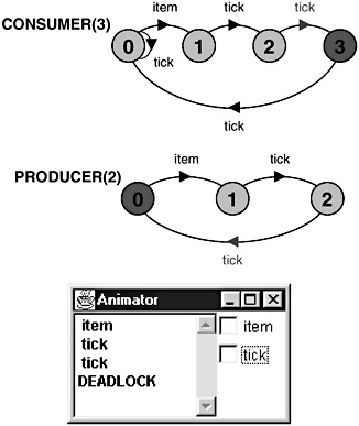
Figure 12.3: Timed Producer – Consumer deadlock.

The deadlock occurs because after the first item is produced and accepted by the consumer, the producer tries to produce another item after two clock ticks, while the consumer must accept a third clock tick before it can accept another item. The deadlock is caused by the timing inconsistency between producer and consumer. The producer is required to produce an item every two seconds while the consumer can only consume an item every three seconds. This kind of deadlock, caused by timing inconsistencies, is termed a time-stop. If we combine processes into a system and time-stop does not occur, we can say that the timing assumptions built into these processes are consistent.

12.1.2 Maximal Progress

Consider a system that connects the PRODUCER and CONSUMER processes of the previous section by a store for items as shown below:

 STORE(N=3) = STORE[0], STORE[i:0..N] = (put -> STORE[i+1]              |when(i>0) get -> STORE[i-1]              ). ||SYS = ( PRODUCER(1)/{put/item}         ||CONSUMER(1)/{get/item}         ||STORE         ).

We would reasonably expect that if we specify that items are consumed at the same rate that they are produced then the store would not overflow. In fact, if a safety analysis is performed then the following violation is reported:

 Trace to property violation in STORE:        put        tick        put        tick        put        tick        put

This violation occurs because the consumer has a choice between getting an item from the store, by engaging in the get action, and engaging in the tick action. If the consumer always chooses to let time pass, then the store fills up and overflows. To avoid this form of spurious violation in timed models, we must ensure that an action occurs as soon as all participants are ready to perform it. This is known as ensuring maximal progress of actions. We can incorporate maximal progress into our timed models by making the tick action low priority. For the example, a system that ensures maximal progress is described by:

 ||NEW_SYS = SYS>>{tick}.

Safety analysis of this system reveals no violations. Maximal progress means that after a tick, all actions that can occur will happen before the next tick. However, even though we assume that actions take a negligible amount of time, it would be unrealistic to allow an infinite number of actions to occur between ticks. We can easily check for this problem in a model using the following progress property, which asserts that a tick action must occur regularly in any infinite execution (see Chapter 7).

 progress TIME = {tick}

The following process violates the TIME progress property because it permits an infinite number of compute actions to occur between tick actions:

 PROG = (start   -> LOOP | tick -> PROG), LOOP = (compute -> LOOP | tick -> LOOP). ||CHECK = PROG>>{tick}.

The progress violation is reported by the analyzer as:

 Progress violation: TIME Path to terminal set of states:     start Actions in terminal set: {compute}

If we include an action that terminates the loop and then engages in a tick action, the progress property is not violated:

 PROG = (start   -> LOOP | tick -> PROG), LOOP = (compute -> LOOP | tick -> LOOP        |end -> tick -> PROG        ).

This may seem strange since the loop still exists in the process. However, the end and compute actions are the same priority and consequently, with the fair choice assumption of Chapter 7, the compute action cannot be chosen an infinite number of times without the end action being chosen. The revised LOOP now models a finite number of iterations. The tick action following end means that the PROG process can only execute this finite LOOP once every clock tick. Consequently, the TIME progress property is not violated.

12.1.3 Modeling Techniques

Incorporating time in models by the simple expedient of a global tick action is surprisingly powerful. In the following, we look at modeling techniques for situations that occur frequently in timed systems.

Output in an Interval

The examples we have seen so far produce an output or accept an input at a precise time, within the limitations of the discrete model of time. The INTERVAL process below produces an output at anytime after Min ticks and before Max ticks. The LTS for the process is depicted in Figure 12.4.

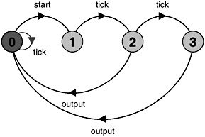
Figure 12.4: LTS for OUTPUT (1,3).

 OUTPUT(Min=1,Max=3) =   (start -> OUTPUT[1] | tick -> OUTPUT), OUTPUT[t:1..Max] =   (when (t>Min && t<=Max) output ->OUTPUT   |when (t<Max)           tick ->OUTPUT[t+1]   ).

The technique of using choice with respect to the tick action allows us to model processes in which the completion time is variable, for example, due to loading or congestion.

Jitter

A variation on the previous technique is a process that periodically produces an output at a predictable rate. However, the output may be produced at any time within the period. In communication systems, this kind of timing uncertainty is termed jitter. The JITTER process defined below is an example of how jitter can be modeled. Figure 12.5 depicts the LTS for the JITTER process.

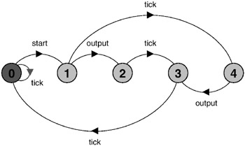
Figure 12.5: LTS for JITTER(2).

 JITTER(Max=2) =   (start -> JITTER[1] | tick -> JITTER), JITTER[t:1..Max] =   (output -> FINISH[t]   |when (t<Max)  tick -> JITTER[t+1]   ), FINISH[t:1..Max] =   (when (t<Max)  tick -> FINISH[t+1]   |when (t==Max) tick -> JITTER   ).

Timeout

Timeouts are frequently used to detect the loss of messages in communication systems or the failure of processes in distributed systems. Java provides a version of the wait() synchronization primitive that takes a timeout parameter – a wait() invocation returns either when notified or when the timeout period expires. The most elegant way to model a timeout mechanism is to use a separate process to manage the timeout, as shown below for a receive operation with a timeout. The timeout and receive processes are combined into a RECEIVER process.

 TIMEOUT(D=1)   = (setTO          -> TIMEOUT[0]     |{tick,resetTO} -> TIMEOUT     ), TIMEOUT[t:0..D]   =(when (t<D) tick      -> TIMEOUT[t+1]    |when (t==D)timeout   -> TIMEOUT    |resetTO              -> TIMEOUT    ). RECEIVE = (start   -> setTO -> WAIT), WAIT    = (timeout -> RECEIVE           |receive -> resetTO -> RECEIVE           ). ||RECEIVER(D=2) = (RECEIVE || TIMEOUT(D))                 >>{receive,timeout,start,tick}                 @{receive,tick,timeout,start}.

In addition to tick, the start, receive and timeout actions are declared as low priority in the RECEIVER composite process. This is because maximal progress requires that an action take place when all the participants in that action are ready. However, the participants in interface actions depend on the system into which RECEIVER is placed, so we should not apply maximal progress to these actions within the RECEIVER process but later at the system level. Consequently, we give interface actions the same priority as the tick action. All internal actions have a higher priority. The minimized LTS for RECEIVER, which hides the internal actions concerned with setting and resetting the timeout, is depicted in Figure 12.6.

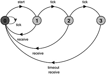
Figure 12.6: LTS for RECEIVER(2).