Section 15.1. Basic Data Grouping | Excel 2007[c] The Missing Manual

15.1. Basic Data Grouping

When you want to simplify your worksheets, you first have to learn how to group data. Grouping data lets you tie related columns or rows into a single unit. Once you've put columns or rows into a group, you can collapse the group, temporarily hiding it and leaving more space for the rest of your data. At its simplest, grouping is just a quick way to help you easily view what you want to see, when you want to see it. It's most handy when you want to show all the key summary information but none of the numbers that you need to crunch to arrive at these results.

Note: Excel's grouping settings also affect how your worksheet prints outcollapsed rows or columns don't appear in your printout.

UP TO SPEED
Comparing Grouping and Tables

Overall, grouping isn't as powerful as Excel's tables (covered in Chapter 14). Whereas tables include features for sorting, filtering, and searching, groups simply try to make it easier to work with data tables that use one or more levels of subtotals.

Of course, there's no reason you can't use both grouping and tables. You may group one or more columns in a big table so that you can see just the columns you want (all the columns that track address components , for instance).

This approach works well if you're grouping multiple columns, but it doesn't work as well if you're grouping rows. Excel tables grow dynamically, so you could have a problem. If you add a new row at the bottom of a table (or a new column on either side), the table automatically expands to incorporate the new information. Groups don't have the same behavior. As a result, if your table grows, some of it may slip out beyond an edge of the group.

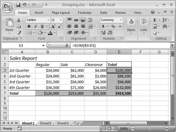
15.1.1. Creating a Group

To see how grouping can simplify complex worksheets, check out the sales report data shown in Figure 15-1. In this example, the information fits easily into the viewable area of the Excel window, but in a real-world company, you could easily end up needing to extend the worksheet with more columns and rows.

Figure 15-1. This worksheet shows the products sold at a retail store, with the numbers broken down in two ways: by quarter, and by the type of merchandise (regular priced, on-sale , and clearance). The data is subtotaled so you can tell how much the company sold in a particular category over the whole year (cells B7:D7), how much it sold in a quarter in all categories ( cells E3:E6), and how much it sold in total ( cell E7).

You could add a variety of columns (representing different types of promotions, different discounts from regular prices, or different departments in the store). Or, you may add more rows to cover sales quarters from more than one year, or to track monthly, weekly, or even daily sales totals. In either case, the data would become fairly unwieldy, forcing you to scroll up and down the worksheet, and from side to side. By grouping columns (or rows) together, you can pop them in and out of view with a single mouse click.

Note: You may remember from Chapter 5 that you can also use hiding to temporarily remove rows and columns from sight. But grouping is a much nicer approachyou can more easily pop data out of and back into view without going hunting through the menu. It also makes it more obvious to the person reading the worksheet that there's more data tucked out of sight. People more often use hiding to remove gunk that no one ever needs to see. Technically, grouping uses Excel's hiding ability behind the scenes to make grouped cells disappear temporarily.

Here are the steps you'd need to follow in order to group several columns together using the sales report example:

Select the columns or rows you want to group .

In most cases, you'll want to group the detail columns that provide fine-grained information (like columns B, C, and D). You shouldn't include in your group any subtotals (like column E) that summarize your information, because you're likely to want to see those subtotals.

To make your selection, drag over the column headers so that you've selected the entire column. This way, Excel can tell right away that you want to group columns. In the sales report example, you'd choose columns B, C, and D.
Choose Data Outline Group .

If Excel isn't sure which groups of cells you want to group, it shows a Group dialog box that lets you specify whether you're grouping columns or rows. (If you selected cells B3:D3, Excel would consider it an ambiguous selection because the selection could represent an attempt to group the columns or rows.) If the Group dialog box appears, make your selection, and then click OK.

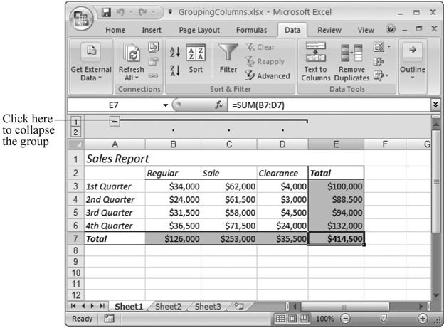
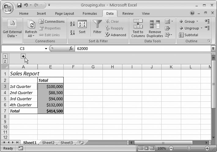
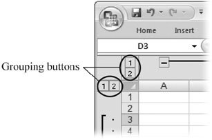
When you group your columns, the worksheet doesn't change, although a new margin area appears at the top of the worksheet, as shown in Figure 15-2. This margin allows you to collapse and expand your groups (see Figure 15-3). To collapse a group, click the minus sign (), which then changes into a plus sign (+). To expand a collapsed group, click the plus sign (+).

To remove a group after you've established it, expand the group, select all the columns, and then choose Data Outline Ungroup. If you select only some of the columns, Excel removes the selected columns from the group, but leaves the rest of the group intactas long as at least two grouped columns remain . (If you remove a column from the middle of a group, youre actually left with two groups, one with the columns on the left, and one with the columns on the right.)

Figure 15-2. Here, columns B, C, and D have been grouped together.

Figure 15-3. After clicking the minus icon in the worksheet's upper margin (as shown in Figure 15-2), you can quickly collapse this group, hiding columns B, C, and D. When you've hidden columns, Excel still uses them in calculations (like those in column E).

Tip: You can also ungroup a set of columns while the group's collapsed. Just select a range of columns that includes the hidden columns, and then use the Data

Outline

Ungroup command. Even though youve removed the group, the columns remain hidden and trapped out of sight! You can expose these columns after you've removed the group only if you select a range of columns that includes the hidden columns, and then choose Home

Cells

Format

Hide & Unhide

Unhide Columns.

Outline

Group. This time, a margin appears just to the left of the worksheet, allowing you to quickly hide the grouped rows. You can also have groups of rows and groups of columns, as shown in Figure 15-4.

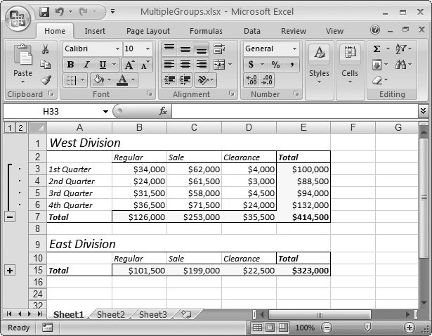
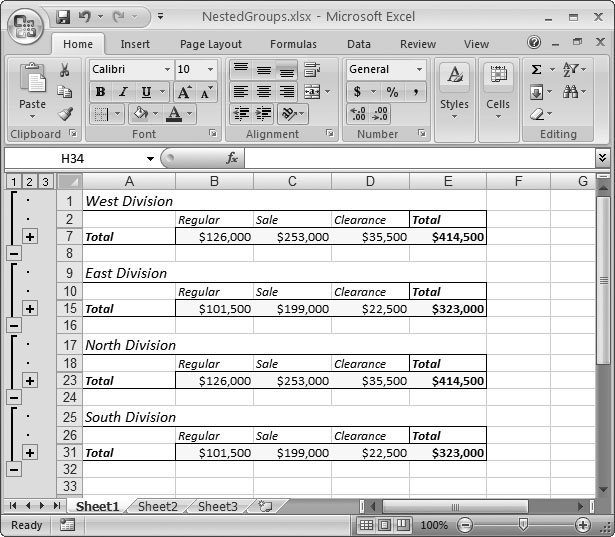
Figure 15-4. The trick to mastering Excel's grouping abilities is understanding how the grouping bars work. The grouping bars show you the range of cells that are bound together in a single group. The minus sign (-) icon always appears just outside the group (either over the column to the left, or under the last row). That's because this icon must remain visible after you've collapsed the group so that you can expand it.

Note: If you insert a new row between two grouped rows using the Home

Cells

Insert

Insert Sheet Rows command, Excel automatically places the new row into the group. The sames true if you insert a new column between two grouped columns using Home

Cells

Insert

Insert Sheet Columns.

Tip: If you decide to use multiple groups, it makes sense to group related rows or columns. For example, you may group all the columns that have address information into one group.

15.1.2. Nesting Groups Within Groups

As you've seen, grouping lets you temporarily shrink the size of a large table by removing specific rows or columns. Grouping becomes even more useful when you create a worksheet that has multiple tables of information, like the one shown in Figure 15-5.

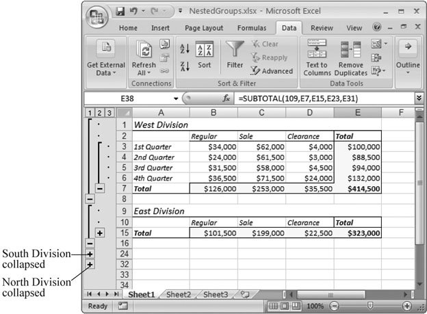
Figure 15-5. This worksheet includes two separate groups with data. Currently, the lower group is collapsed, so that you see only the totals. Thanks to grouping, you can fill a worksheet with dozens of separate tables with detailed information, but you can still see the summary information for them all when you collapse the groups.

Note: Don't get confused by thinking about Excel's structured tables, which you saw in Chapter 14. With grouping, you can use any combination of cells. Here, the data falls into a tabular structure with easily identifiable rows and columns, but it isn't an official Excel table.

Not only can you create separate groups for different tables, you can also put one group inside another. This approach gives you multiple viewing levels. Consider Figures 15-6 and 15-7, which show two views of the same worksheet. This worksheet includes four tables, each of which has two levels of grouping. By collapsing the first-level group for a table, you can hide everything except the summary information (listed in the Total line). By collapsing the second-level group, you can hide the entire table.

Figure 15-6. All four tables are partially collapsed, and each has its second-level groups hidden so that they show just the total sales information for each region.

Figure 15-7. You see only two tables. The West Division is completely visible because both its levels are expanded. The East Division is partially visible because its second-level group is collapsed. The North and South Division tables aren't visible at all because the first-level group for each table is collapsed.

Note: The only drawback is that the more levels of grouping you add, the more room Excel needs in the margins at the side of the worksheet in order to display all the grouping lines.

Technically, when you add more than one level of grouping, you're adding collapsible outline views to your worksheet, which let you quickly move back and forth between a bird's-eye view of your data and an up-close glimpse of multiple rows.

TIMESAVING TIP
Collapsing and Expanding Multiple Groups at Once

If you create a worksheet with multiple levels of grouping, you can find yourself doing a lot of clicking to expose all the information you're interested in (or to hide all the details you don't care about). Fortunately, Excel includes a helpful shortcut that lets you expand or collapse multiple groups at once: grouping buttons (shown in Figure 15-8).

Each grouping button is labeled with a number. If you click number 1, Excel collapses all the column or row groups. If you click number 2, Excel collapses all the groups except the top level. If you click number 3, Excel collapses all the groups except the first two levels, and so on. In the sales worksheet shown in Figure 15-7, you can click 3 to show the whole worksheet, 2 to show just the subtotals, or 1 to hide all the sales tables.

Excel displays a different number of grouping buttons, depending on your worksheet's levels of grouping. The largest numbered button you'll see is 8, because Excel allows a maximum of seven levels of nested groups.

Figure 15-8. Excel provides two sets of grouping buttons: one for row grouping (just above the row numbers), and one for column grouping (just to the left of the column letters ).

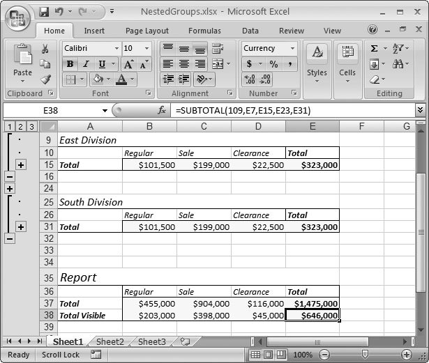
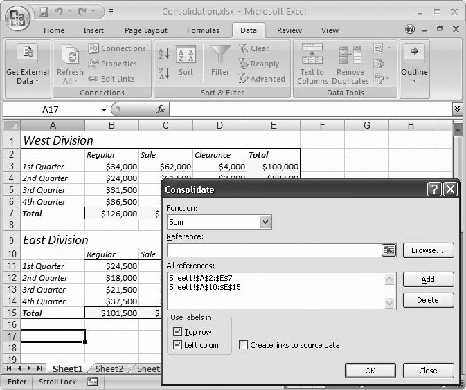
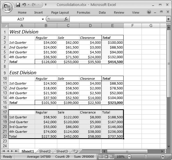
15.1.3. Summarizing Your Data

Understanding how to quickly collapse and expand tables is all well and good, but before long, you'll want to add up the totals you've collected in these accordionstyle tables. In the subtotaled sales report shown in Figure 15-7, the perfect way to complete this worksheet is to add a final table that sums up all the Total rows listed in the last row of each division.

To create a grand summary, you need to employ just a few more formulas. These formulas add the separate subtotals (contained in columns B, C, D, and E) to arrive at a final series of grand totals. The following formula would calculate the total sales in all divisions and all quarters for regular merchandise:

 =B7+B15+B23+B31

Note: You could, of course, also calculate any of these subtotals by using the SUM( ) function, which is covered in Section 9.2.

You'll notice that no matter how you expand or collapse the groups in your worksheet, the result of these formulas is always the same. That's because, whether you're using straight addition (of multiple cells) or the SUM( ) function, Excel takes into account visible and hidden cells. If you're using grouping, however, it may occur to you that it would be handy if you could perform a calculation that deals only with the visible cells. That way, you could choose the portions of a worksheet you want to consider, and the formula could recalculate itself automatically to give you the corresponding summary information.

Good news: Excel gives you the power to build this sort of formula. All you need is the awesome SUBTOTAL( ) function. As you may recall from Chapter 14, the SUBTOTAL ( ) function is a useful tool for calculating totals in filtered lists. But it's just as helpful when you apply it to outlines because it ignores collapsed rows and columns.

As explained in Section 14.4.5, the first argument (known as the calculation code) you use with the SUBTOTAL( ) function tells Excel the type of math you want to do (summing, averaging, counting, and so on). If you want to ignore the hidden cells in collapsed groups, you have to use the calculation codes above 100. If you want to perform a sum operation, then you need to use the code 109. (For a full list of the SUBTOTAL( ) calculation codes, see Section 14.4.6.)

Once you've chosen the calculation code, you need to specify the cells or range of cells you want to add. Here's an example that rewrites the earlier formula to sum only visible cells:

 =SUBTOTAL(109,B7,B15,B23,B31)

Figure 15-9 shows the difference between using the SUBTOTAL( ) function and the SUM( ) function.

15.1.4. Combining Data from Multiple Tables

Instead of writing your summary formulas by hand, you can generate a summary table automatically that takes advantage of Excel's ability to consolidate data. Consolidation works if you have more than one table with precisely the same layout. You can use consolidation to take the different tables shown in the sales report (West Division, East Division, and so on) and calculate summary information. Excel creates a new table that has the same structure but combines the data from the other tables. You can choose how Excel combines the data, including whether the numbers should be totaled, averaged, multiplied, and so on.

Note: Data consolidation works with any sort of tabular data. You don't need to create the structured tables you learned about in Chapter 14.

Figure 15-9. This worksheet calculates summary information using two different approaches. The formulas in row 37 use the SUM( ) function, while the formulas in row 38 use the SUBTOTAL( ) function. In the SUBTOTAL( ) calculation, Excel doesn't use the subtotals for the completely hidden tables, giving a different result than that provided by the SUM( ) function.

Data consolidation works with any worksheet (with or without grouping); you can even use it to analyze data in identically structured tables from different worksheets.

Note: For best results, you should consolidate data with the exact same layout only. Although you can coax Excel into combining differently sized ranges of data, it's all too easy to confuse yourself about what is and isn't combined. To make life easier, only consolidate ranges that have numeric data or identical labels (like column or row titles). Leave out the overall table title because there's no way to consolidate it.

To consolidate the sales report data, follow these steps:

Move to the location where you want to insert the summary table .

Excel inserts the summary table, starting at the current cell. Make sure you've scrolled down past all your data, so you don't overwrite important information.
Choose Data Data Tools Consolidate .

The Consolidate dialog box appears, as shown in Figure 15-10.

From the Function pop-up menu, choose how you want to combine numbers .

In the sales report, Sum is the best choice to calculate total sales. However, you may want to create separate tables that pick out the best or worst sales using Max and Min.

Figure 15-10. This worksheet contains two detailed sales tables that are about to be consolidated. Both ranges have been added to the Consolidate dialog box (they're listed in the "All references" list), and the "Top row" and "Left column" checkboxes have been turned on so that Excel can find and use the headings on either side of the table.

Click inside the Reference text box. Now, drag to select the first table you want to consolidate in the worksheet .

If Excel's main window isn't already visible, click the icon at the right end of the Reference text box to collapse the Consolidate dialog box. You have to click this icon again to restore the window when you're done selecting the cells you want.
Once you've selected the appropriate cells, click the Consolidate dialog box's Add button .

The range appears in the "All references" list.
Return to step 4 to select the next table you want to consolidate .

Repeat steps 4 and 5 for each table you want to consolidate.
If your selection includes labels (like row or column titles), select the "Top row" or "Left column" checkbox to tell Excel where the labels are .

If you don't tell Excel where the labels are, it ignores these cells, and the corresponding cells in the summary table wind up blank. But if you use these checkboxes to tell Excel where the labels are, Excel simply copies the labels directly to the summary table.

Note: If the labels don't match exactly in the ranges you're using, you may need to clear the "Top row" and "Left column" checkboxes to perform your consolidation. Otherwise, depending on the placement of these labels, Excel may refuse to consolidate your data.

Click OK to generate the summary table .

When creating the consolidated data, Excel copies headings and calculates numbers, but it doesn't copy any of the source formatting. Figure 15-11 shows the result.

Figure 15-11. Here, the newly created consolidated data table is at the bottom of the worksheet. In this case, someone used the Sum option, which means that the consolidated data shows the totals you get by adding the values from the separate tables. Cell B18 has the consolidated data for regularly priced merchandise sold in the first quarter in both the West and East Divisions (cells B3 and B11).

Data consolidation's big disadvantage is that it generates a table filled with numbers, rather than formulas. Microsoft's engineers probably designed the consolidation feature this way so you can consolidate data from multiple files and not worry about losing the information if the source files move or their structure changes.

But this behavior means that if you modify any of the sales figures, the summary table doesn't update. Instead, you'll need to generate a completely new summary table by using the Data Data Tools Consolidate command. Fortunately, the second time around should be quite a bit faster, because Excel keeps track of all the ranges youve selected for consolidation, so you don't need to define them again.