7.2. Formula Shortcuts So far, you've seen how to build a formula by typing it in manually. That's a great way to start out, because it helps you to understand the basics of formula writing. But writing formulas by hand is a drag; plus, it's easy to type in the wrong cell address. For example, if you type A2 instead of A3, you can end up with incorrect data, and you won't necessarily notice your mistake right away. And what about writing formulas for really basic math functions, like calculating the average of a column of numbers? There's no sense in reinventing the wheel, so Excel offers a bunch of canned functions you can use to build your formulas. As you become more comfortable with formulas, you can start taking advantage of the formula tools Excel gives youlike point-and-click formula creation and the Insert Function buttonto speed up your formula writing and reduce your mistakes. You'll learn about these features in the following sections. 7.2.1. Point-and-Click Formula Creation Instead of entering a formula by typing it out letter by letter, Excel lets you create formulas by clicking the cells you want to use. For example, here's a simple formula that totals the numbers in two cells: =A1+A2
To build this formula by clicking, just follow these steps: Move to the cell where you want to enter the formula. This cell is where the result of your formula's calculation appears. While you can pick any cell on the worksheet, A3 works nicely because it's directly below the two cells you're adding. Press the equal sign (=) key. The equal sign tells Excel you're going to enter a formula. Move to the first cell you want to use in your formula (in this case, A1). You can move to this first cell by pressing the up arrow key twice, or by clicking it with the mouse. You may notice that moving to another cell doesn't cancel your edit, as it would normally, because Excel recognizes that you're building a formula. When you move to the new cell, the cell reference appears automatically in the formula (which Excel displays in cell A3, as well as in the Formula Bar just above your worksheet). If you move to another cell, Excel changes the cell reference accordingly. Add the + sign to your formula by pressing the + key. Excel adds the + sign to your formula so that it now reads =A1+. Finish the formula by moving to cell A2 and pressing Enter. Again, you can move to A2 either by pressing the up arrow key or by clicking the cell directly. Remember, you can't just finish the formula by moving somewhere else; you need to press Enter to tell Excel you're finished writing the formula. Another way to complete your edit is to click the checkmark that appears on the Formula Bar, to the left of the current formula. Forgetting to complete a formula is a common source of frustration, even for experienced Excel fans. If you click another cell before you press Enter, you don't move to the cellinstead, Excel inserts the cell into your formula.
Tip: You can use this technique to create any formula. Just type in the operators, function names, and so on, and use the mouse to select the cell references. If you need to select a range of cells, just drag your mouse until the whole group of cells is highlighted. You can practice this technique with the SUM( ) function. Start by typing =SUM( into the cell, and then selecting the range of cells you want to add. Finish by adding a final closing parenthesis and pressing Enter.
7.2.2. Point-and-Click Formula Editing You can use a similar approach to edit formulas, although editing formulas is slightly trickier. Move to the cell that contains the formula you want to edit, and put it in edit mode by double-clicking it or pressing F2. Excel highlights all the cells that this formula uses with a colored outline. Excel is even clever enough to use a helpful color-coding system. Each cell reference uses the same color as the outline surrounding the cell it's referring to. This color coding can help you pick out where each reference is. Click the outline of the cell you want to change. (Your pointer changes from a fat plus sign to a four-headed arrow when you're over the outline.) With your mouse button still held down, drag this outline over to the new cell(s) you want to use. Excel updates the formula automatically. You can also expand and shrink cell-range references. To do so, put the formula-holding cell into edit mode, and click the bottom-left corner of the border surrounding the range you want to change. Next, drag the border to change the size of the range. If you want to move the range, click any part of the range border and drag the outline the same way you would with a cell reference. Press Enter or click the Formula bar checkmark to tell Excel you're finished editing. That's it.
7.2.3. Using the Insert Function Button to Quickly Find and Use Functions Excel provides more than 500 useful built-in functions. In order to use a function, however, you need to type its name in exactly. That means that every time you want to employ a function, you need to refer to this book, call on your own incredible powers of recollection, or click over to the convenient Insert Function button. FREQUENTLY ASKED QUESTION
Showing and Printing Formulas | How in the world do I print out formulas that appear in my cells? When you print a worksheet, Excel prints the calculated value in each cell rather than any formula that happens to be inside a cell. Usually, that's what you want to have happen. But in some cases, rather than a printout of the formula's results, you want a record of the calculations Excel uses to generate the results. No problem. Excel provides a view setting that makes this possible. Just choose Tools  Options from the Excel menu, and select the View tab. Then, turn on the Formulas checkbox, and click OK. Now, Excel displays the formulas contents instead of its results. Turn off the Formulas checkbox to return to normal mode. Options from the Excel menu, and select the View tab. Then, turn on the Formulas checkbox, and click OK. Now, Excel displays the formulas contents instead of its results. Turn off the Formulas checkbox to return to normal mode. |
When you click this button (labeled fx, just to the right of the Formula bar), Excel displays the Insert Function dialog box (shown in Figure 7-5), which offers three ways to search for and insert any of Excel's functions: Any functions you've previously used appear in the text box below "Select a function." If you're looking for a function, the easiest way to find one is to choose a category from the "Select a category" pull-down menu. For example, if you select the Math & Trig category, you'll see a list of functions with names like SIN( ) and COS( ), which perform basic trigonometric calculations. If you're really ambitious, you can type a couple of keywords into the "Search for a function" text box. Next, click Go to perform the search. Excel gives you a list of functions that match your keywords.
Figure 7-5. Use the Insert Function dialog box to find the function you need. When you click one of the functions in the list, Excel gives you a description of it at the bottom of the window. 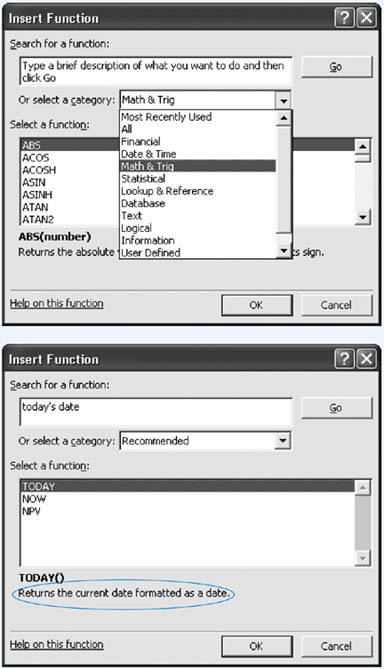
When you spot a function that looks promising, click it once to highlight its name. Excel then displays a brief description of the function at the bottom of the window. For more information, you can click the "Help on this function" link in the bottom-left corner of the window. To build a formula using this function, click OK. Excel then inserts the function into the currently active cell, followed by a set of parentheses. Next, it closes the Insert Function dialog box and opens the Function Arguments dialog box (Figure 7-6). Figure 7-6. Top: The Function Arguments dialog box walks you through the process of inserting a function into a formula. Because the COMBIN( ) function requires two arguments (Number and Number_chosen), the Function Arguments dialog box shows two text boxes.
Bottom: If you need more room to see the worksheet and select cells, you can click the Collapse Dialog Box icon to reduce the window to a single text box. Clicking the Expand Dialog Box icon restores the window to its normal size. 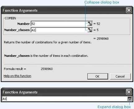
Note: Depending on the function you're using, Excel may make a (somewhat wild) guess about which arguments you want to supply. For example, if you use the Insert Function window to add a SUM( ) function, you see that Excel picks a nearby range of cells. If this isn't what you want, just replace the suggest range with the values you want.
Now you can finish creating your formula by using the Function Arguments dialog box, which includes a text box for every argument in the function. As you enter the arguments, Excel updates the formula in the worksheet's active cell and displays the result of the calculation at the bottom of the Function Arguments dialog box. The Function Arguments dialog box also includes a help link ("Help on this function") you can click to get detailed information about the function. As shown in Figure 7-7, Excel's help page includes a brief description of the function, important notes, and a couple of sample formulas that use the function, complete with results. To complete your formula, follow these steps: Click the text box for the first argument. A brief sentence describing the argument appears in the Function Arguments dialog box. Some functions don't require any arguments. If this is the case, you don't see any text boxes, although you still see some basic information about the function. Skip directly to step 4. Enter the value for the argument. If you want to enter a literal value (like the number 52), type it in now. To enter a cell reference, you can type it in manually or click the appropriate cell on the worksheet. To enter a range, drag the cursor to select a group of cells. You may need to move the Function Arguments dialog box to the side to expose the part of the worksheet you want to click. The Collapse Dialog Box icon (located to the immediate right of each text box) is helpful, since clicking it shrinks the window's size. This way, you'll have an easier time selecting cells from your worksheet. To return the window to normal, click the Expand Dialog Box icon, which appears to the right of the text box. Figure 7-7. The help page shown here shows the reference for the trigonometric SIN( ) function, which calculates the sine of an angle. 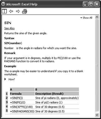 Repeat step 2 for each argument in the function. As you enter the arguments, Excel updates the formula automatically. Once you've specified a value for every argument, click OK. Excel closes the window and returns you to your worksheet.
|