Section 7.1. Creating a Basic Formula
7.1. Creating a Basic FormulaFirst things first: what exactly do formulas do in Excel? A formula is simply a series of mathematical instructions that you place in a cell in order to perform some kind of calculation. These instructions may be as simple as telling Excel to add up (sum) a column of numbers, or they may be complex enough to use advanced statistical functions to spot trends and make predictions. Here are some sample formulas written in English (the rest of this chapter is devoted to writing formulas in Excel-speak):
As you can imagine, formulas are outrageously useful, no matter what kind of spreadsheet you're creating. Say, for example, you're in sales, and you want to create a spreadsheet that keeps track of your yearly income and expenses. You can type in your sales figures for the last month and have Excel calculate and display updated year-to-date sales and profit figuresinstantly. Or, imagine that you want to create a spreadsheet to track the housing market. (You're thinking of buying a house, and you want to compare prices, mortgage rates, and loan terms on a bunch of different properties to see if you can afford anything you'd actually want to live in.) Using formulas, you can run instant "what if" calculations that show how a dozen projected monthly payments would be affected if you went with a 30-year loan over a 15-year loan. Cool, huh? In Excel, all formulasfrom dead-simple to scientist-scaryshare the same basic characteristics. Here are a few points to note:
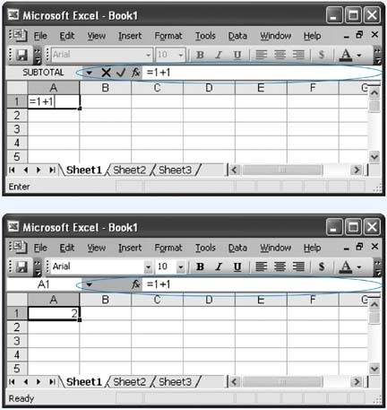
One of the simplest formulas you can create is this one, shown in Figure 7-1: =1+1 The equal sign is how you tell Excel that you're entering a formula (as opposed to a string of text or numbers). The formula that follows the equal sign is what you want Excel to calculate. Figure 7-1. Top: This simple formula begins its life when you type it into a cell. To complete your formula and tell Excel to display the result, either press Enter, or head to the Formula bar and click the checkmark. (Clicking the X button that appears to the left of the Formula bar cancels the formula). |
OPERATOR | NAME | EXAMPLE | RESULT |
|---|---|---|---|
+ | Addition | =1+1 | 2 |
- | Subtraction | =1-1 | 0 |
* | Multiplication | =2*2 | 4 |
/ | Division | =4/2 | 2 |
^ | Exponentiation | =2^3 | 8 |
% | Percent | =20% | 0.20 |
Numbers. These old friends1, 2, 3, and so onare known in formula-speak as constants or literal values, because they never change (unless you edit the formula).
Cell references. These references point to another cell (for example, $A$5), or a range of cells (for example, B1:B25), that you need data from in order to perform a calculation. For example, say you have a list of 10 house prices. A formula in the cell beneath this list can refer to all 10 of the cells above it in order to calculate the average house price.
Functions. Functions are specialized formulas, built into Excel, that let you perform a wide range of calculations. For example, Excel provides dedicated functions that calculate sums and averages, standard deviations, yields, cosines and tangents, and much more. These functions span every field from financial accounting to trigonometry, so there's something for everyone.
Spaces. Excel ignores spaces. However, you can use them to make a formula easier to read. For example, you can write the formula =3*5 + 6*2 instead of =3*5+6*2. (The only exception to this ignoring-spaces rule occurs with cell ranges, where spaces do have a special meaning.)
Note: The percentage (%) operator divides a number by 100.
7.1.1. Excel's Order of Operations
For computer programs and human beings alike, one of the basic challenges when it comes to reading and calculating formula results is figuring out the order of operationsmathematician-speak for deciding which calculations to perform first when there's more than one calculation in a formula. For example, take a look at this formula:
=10 - 8 * 7
Do you subtract the 8 from the 10 first, or multiply the 8 times the 7 first? Your choice matters: the result, depending on your order of operations, is either 14 or -46. Fortunately, Excel abides by what's come to be accepted among mathematicians as the standard rules for order of operations, meaning it doesn't necessarily process your formulas from left to right. Instead, it evaluates complex formulas piece by piece in this order:
Parentheses (any calculations within parentheses are always performed first)
Percent
Exponents
Division and multiplication
Addition and subtraction
Note: If Excel encounters formulas that contain operators of equal precedencethat is, the same order-of-operation priority levelit evaluates these operators from left to right. (Excel could just as easily choose right, since it doesn't make a difference to basic mathematical formulas.)
For example, take a look at the following formula:
=5 + 2 * 2 ^ 3 - 1
To arrive at the answer of 20, Excel first performs the exponentiation (2 to the power of 3):
=5 + 2 * 8 - 1
and then the multiplication:
=5 + 16 - 1
and then the addition and subtraction:
=20
To change the order Excel follows, you can add parentheses. For example, notice how adding parentheses affects the result in the following formulas:
5 + 2 * 2 ^ (3 - 1) = 13 (5 + 2) * 2 ^ 3 - 1 = 55 (5 + 2) * 2 ^ (3 - 1) = 28 5 + (2 * (2 ^ 3)) - 1 = 20
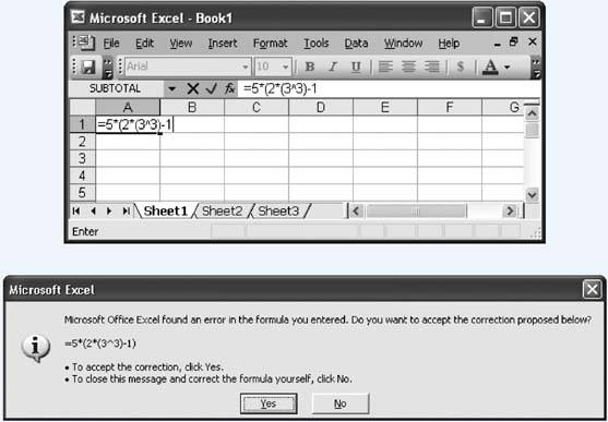
You must always use parentheses in pairs (one open parenthesis for every closing parenthesis). If you don't, Excel gets confusedand lets you know it's confused by displaying a dialog box (Figure 7-2). In the dialog box, you find Excel's best guess for correcting the formula. If the suggestion looks good, click Yes to accept it; otherwise, click Cancel to banish the dialog box and edit your formula by hand.
Figure 7-2. Top: If you create a formula with a mismatched number of opening and closing parentheses (like this one), Excel politely lets you know by displaying the dialog box at bottom.
Bottom: Excel offers to correct the formula by adding the missing parenthesis at the end. You may not want that, though. If not, cancel the suggestion, and edit your formula by hand.
As you edit your formula by hand, Excel helps a little bit by highlighting matched sets of parentheses. For example, as you move to the opening parenthesis, Excel automatically bolds both the opening and closing parentheses in the Formula bar, so you can easily identify the expression that's enclosed between them.
7.1.2. Cell References
Excel's formulas are handy when you want to perform a quick calculation. But if you want to take full advantage of Excel's power, you're going to want to use formulas to perform calculations on the information that's already in your worksheet. To do that you need to use cell referencesExcel's way of pointing to, or referencing, one or more cells in a worksheet.
For example, you may want to calculate the cost of your Amazonian adventure holiday based on information like the number of days your trip will last, the price of food and lodging, and the cost for vaccination shots at a travel clinic. If you use cell references, you can enter all this information into different cells and then write a formula that calculates a grand total. This approach buys you unlimited flexibility, because you can change the cell data whenever you want (for example, turning your three-day getaway into a month-long odyssey), and Excel will refresh the formula results automatically.
Cell references are a great way to save a ton of time. They come in handy when you want to create a formula that involves a handful of widely scattered cells whose values frequently change. For example, rather than manually adding up a bunch of subtotals to create a grand total, you can create a grand-total formula that uses cell references to point to a handful of subtotal cells. Cell references also let you refer to large groups of cells by specifying a range. For example, using the cell-reference lingo you learn in the upcoming section "Specifying Cell Ranges" (Section 7.1.5), you can specify all the cells in the first column between the 2nd and 100th rows.
Every cell reference points to another cell. For example, if you want a reference that points to cell A1 (the cell in column A, row 1), use this cell reference:
=A1
In Excel-speak, this reference translates to "get the number from cell A1, and insert it in the current cell." So if you put this formula in cell B1, it displays whatever value is currently in cell A1. In other words, these two cells are now linked.
Cell references work within formulas just as regular numbers do. For example, the following formula calculates the sum of two cells, A1 and A2:
=A1+A2
Provided both cells contain numbers, you see the total appear in the cell that contains the formula. (If one of the cells doesn't contain numeric information, you see a special error code instead that starts with a # symbol. Errors are described in more detail on Section 7.1.6.)
7.1.3. How Excel Formats Cells that Contain Cell References
As you learned in Chapter 4, the way you format a cell affects how Excel displays the cell's value. When you create a formula that references other cells, Excel attempts to simplify your life by applying automatic formatting. It reads the number format that the source cells (i.e., the cells being referred to) use, and applies that to the cell with the formula. This means that if you add two numbers and you've formatted both with the Currency number format, your result also has the Currency number format. Of course, you're always free to change the formatting of the cell after you've entered the formula.
Usually, Excel's automatic formatting is quite handy. Like all automatic features, however, it's a little annoying when it springs into action if you don't understand how it works. Here are a few points to consider:
Excel copies only the number format to the formula cell. It ignores other details, like fonts, fill colors, alignment, and so on. (Of course, you can manually copy formats using the Format Painter, as discussed on Section 4.3.3.)
If your formula uses more than one cell reference and the different cells use different number formats, Excel uses its own rules of precedence to decide which number format to use. For example, if you add a cell that uses the Currency number format with one that uses the Scientific number format, the destination cell has the Scientific number format. Sadly, these rules aren't spelled out anywhere, so if you don't see the result you want, the best approach is just to set your own formatting.
If you change the formatting of the source cells after you've entered the formula, your new formatting doesn't have any effect on the formula cell.
Excel copies source cell formatting only if the formula cell originally uses the General number format (which is the format that all cells begin with). If you apply another number format to the formula cell before you enter the formula, Excel doesn't copy any formatting from the source cells. Similarly, if you change a formula to refer to new source cells, Excel doesn't copy the format information from the new source cells.
| GEM IN THE ROUGH Excel Is a Pocket Calculator |
Sometimes you need to calculate a value before you enter it into your worksheet. Before you reach for your pocket calculator, you may be interested to know that Excel lets you enter a formula in a cell, and then use the result in that same cell. This way, the formula disappears, and you're left with the result of the calculated value. Start by typing your formula into the cell (for example =65*88). Then, press F2 to put the cell into edit mode. Next, press F9 to perform the calculation. Finally, just hit Enter to insert this value into the cell Remember, when you use this technique, you replace your formula with the calculated value. That means if your calculation is based on the values of other cells, Excel doesn't update the result if you change those other cells' values. That's the difference between a cell that has a value and a cell that has a formula. |
7.1.4. Functions
A good deal of Excel's popularity is due to the collection of functions it provides. Functions are built-in, specialized algorithms that you can incorporate into your own formulas to perform powerful calculations. Functions work like miniature computer programsyou supply the data, and the function performs a calculation and gives you the result.
In some cases, functions just simplify calculations that you could probably perform on your own. For example, most people know how to calculate the average of several values, but if you're feeling a bit lazy, Excel's built-in AVERAGE( ) function automatically gives you the average of any cell range. Even better, Excel functions perform feats that you probably wouldn't have a hope of coding on your own, including complex mathematical and statistical calculations, like calculating a best-fit trendline.
Note: Excel provides a detailed function reference that lists all the functions you can use (and how to use them). This function reference doesn't exactly make for light reading, though; for the most part, it's written in IRS-speak. You'll learn more about using this reference in "Using the Insert Function Button to Quickly Find and Use Functions" on Section 7.2.3.
Every function provides a slightly different service. For example, one of Excel's statistical functions is named COMBIN( ). It's a specialized tool used by probability mathematicians to calculate the number of ways a set of items can be combined. You may think this sounds technical, but even ordinary folks can use COMBIN( ) to get some interesting information. You can use the COMBIN( ) function, for example, to count the number of possible combinations there are in certain games of chance.
The following formula uses COMBIN( ) to calculate how many different five-card combinations there are in a standard deck of playing cards:
=COMBIN(52,5)
Note: Functions alone don't actually do anything in Excel. They need to be part of a formula to produce a result. For example, COMBIN( ) is the name of a function. But it actually does somethingthat is, it gives you a resultonly when you've inserted it into a formula, like so: =COMBIN(52,5).
Whether you're using the simplest or the most complicated function, the syntaxor, rules for including a function within a formulais always similar. To use a function, simply enter the function name, followed by parentheses. Then, inside the parentheses, put all the information that particular function needs in order to perform its calculations.
In the case of the COMBIN( ) function, COMBIN( ) requires two pieces of information, or arguments. The first is the number of items in the set (the 52-card deck), and the second is the number of items you're randomly selecting (in this case, 5). Most functions, like COMBIN( ), require two or three arguments. But there's no magic number. Some functions can accept many more, while a few don't need any arguments at all.
Once you've typed the formula =COMBIN(52,5) into a cell, the result (2598960) appears in your worksheet. In other words, there are 2,598,960 different possible five-card combinations in any deck of cards. Rather than having to calculate this fact using probability theoryor, heaven forbid, trying to count out the possibilities manuallythe COMBIN( ) function handled it for you, at lightning speed.
When you enter a function's arguments, be sure to separate each argument with a comma. Excel guides you in this process by providing a tooltipa small pop-up windowthat presents the name of each argument as soon as it recognizes that you're entering a function. For example, when you type =COMBIN and then an open parentheses, Excel displays COMBIN(number, number_chosen) to let you know what information needs to come next. The argument you're currently entering is shown bolded in the tooltip. You don't need to worry about the capitalization of function names, as Excel automatically capitalizes whatever you type in, provided that what you type in matches a known function.
Note: Even if a function doesn't take any arguments, you still need to supply an empty set of parentheses after the function name. One example is the RAND( ) function, which generates a random fractional number. The formula =RAND( ) works fine, but if you forget the parentheses and merely enter =RAND, Excel displays an error message (#NAME?) that is Excelian for: "Hey! You got the function's name wrong." See Table 7-2 on Section 7.1.4 for more information about Excel's error messages.
More complex formulas combine functions, cell references, and numbers. You may even use multiple functions at once. For example, using the five-card combination formula (mentioned above), you can calculate the probability of getting the exact hand you want in one draw:
=1/COMBIN(52,5)
7.1.5. Specifying Cell Ranges
In many cases, you won't want to refer to just a single cell, but rather a range of cells. A range is simply a grouping of multiple cells. These cells can be next to each other (say, a range that includes all the cells in a single column), or they can be scattered across your worksheet. Ranges are useful for computing averages, totals, and many other calculations.
To group together a series of cells into a range, use one of the following three reference operators:
The comma (,) separates more than one cell. For example, the series A1,B7,H9 is a cell range that contains three cells. The comma is known as the union operator. You can add spaces before or after a comma, but Excel just removes them.
The colon (:) separates the top-left and bottom-right corners of a block of cells. For example, A1:A5 is a range that includes cells A1, A2, A3, A4, and A5. The range A2:B3 is a grid that contains cells A2, A3, B2, and B3. The colon is known as the range operatorby far the most powerful way to select multiple cells. You can add spaces before or after the colon, but Excel just removes them.
The space can find cells that are common to two or more different cell ranges. For example, the expression A1:A3 A1:B10 is a range that consists of only three cells: A1, A2, and A3 (because those three cells are the only ones found in both ranges). The space is technically known as the intersection operator, and not too many folks find it useful.
Note: As you might expect, Excel lets you specify ranges by selecting cells with your pointer, instead of typing in the range manually. You see this approach later in this chapter in the "Point-and-Click Formula Creation" section on Section 7.2.
You can't enter ranges directly into formulas that just use the simple operators. For example, the formula =A1:B1+5 doesn't fly. But many functions are happy to accept ranges. For instance, one of Excel's most basic functions is named SUM. SUM calculates the total for a group of cells. To use the SUM( ) function, you must enter its name, an open parenthesis, the cell range you want to add up, and then a closed parenthesis.
Here's how you use the SUM( ) function to add together the three cells A1, A2, and A3:
=SUM(A1, A2, A3)
And here's a more compact syntax that performs the same calculation using the range operator:
=SUM(A1:A3)
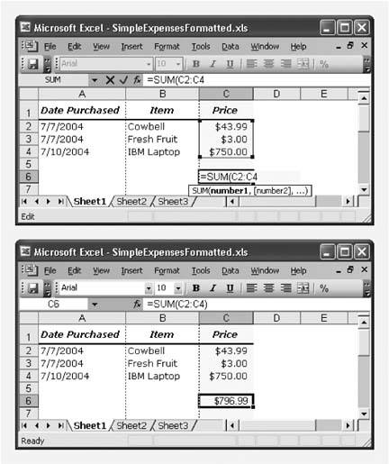
Figure 7-3 shows a similar SUM( ) calculation. Clearly, if you want to total a column with hundreds of values, it's far easier to specify the first and last cell using the range operator rather than to type in each individual cell reference in your formula!
Tip: Sometimes your worksheet has a list with unlimited growth potential, like a list of expenses or a catalog of products. In this case, you can code your formulas to include an entire columnno matter how big it getsby leaving out the row number. For example, the range A:A selects all the cells in column A (and the range 2:2 selects all the cells in row 2). Specifying a range this way also includes any heading cells, which isn't a problem for the SUM( ) function (because it ignores text cells). If you don't want to include the top cell, just create a normal range that stretches to the last cell. For example, to select every cell in column A except for the first one, use the range A2:A65536.
7.1.6. Formula Errors
If you make a syntax mistake when entering a formula (such as leaving out a function argument or including a mismatched number of parentheses), Excel alerts you immediately. Moreover, Excel won't accept the formula until you've corrected it. It's also possible, though, to write a perfectly legitimate formula that doesn't actually generate a valid answer. Here's an example:
Figure 7-3. Top: Using a cell range as the argument in the SUM( ) function is a quick way to add up numbers in a column. When you type a function name that Excel recognizes, a tooltip appears indicating what arguments the function requires. If you're entering a range, as in this example, you'll also see that Excel highlights the cells within the range (C2, C3, and C4) using a blue border.
Bottom: Hitting Enter completes the formula and displays the result.
=A1/A2
If both A1 and A2 have numbers, this formula works without a hitch. But if you leave A2 blank, or if you type text into A2 instead of numbers, Excel can't evaluate the formula, and it reminds you with an error message.
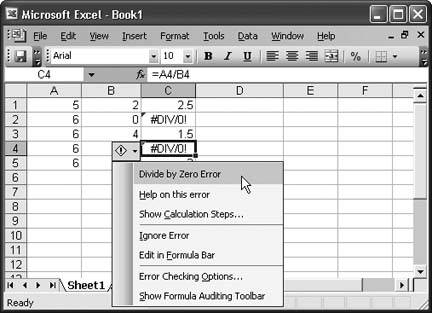
Excel alerts you to formula errors by using special error codes that begin with the number sign (#). As you can see in Figure 7-4, the instant Excel spots an error, it gives you options for fixing it.
Figure 7-4. If Excel spots an error, it inserts a tiny green triangle into the top-left corner of the cell. When you move to the offending cell, Excel displays an exclamation mark next to it. Hover over the exclamation mark to view a description of the error (which appears in a tooltip), or click the exclamation icon to see a list of menu options. Using the menu, you can jump to Excel's online help for tips on fixing the problem.
In order to fix an error, of course, you need to track down the problem and resolve itwhich usually means correcting the formula or changing the cells the formula references. In addition to Excel's error descriptions and online help, you can use the error-code descriptions in Table 7-2 to help you pinpoint the cause of an error and fix it.
Note: Sometimes an error isn't really an error, but simply the result of not typing in all the data your formula references. In this case, you can solve the problem by using a conditional error-trapping formula. This conditional formula checks to see if the data is present and only performs the calculation if it is. The next section, "Logical Operators," shows one way to use an error-trapping formula.
ERROR CODE | DESCRIPTION |
|---|---|
#VALUE! | You used the wrong type of data. Maybe your function expects a single value, and you submitted a whole range. Or, more commonly, you may have used a function or created a simple arithmetic formula with a cell that contains text instead of numbers. |
#NAME? | Excel can't find the name of the function you used. This error usually means you misspelled a function's name, although it may indicate you used text without quotation marks or left out the empty parentheses after the function name. |
#NUM! | There's a problem with one of the numbers you're using. For example, this error appears if a calculation produces a number that's too large or too small for Excel to deal with. |
#DIV/0 | You tried to divide by zero (which, mathematically speaking, is illegal). This error also occurs if you try to divide by a cell that's blank, because Excel treats a blank cell as though it contains the number 0 for the purpose of simple calculations with the arithmetic operators. (Some functions, like AVERAGE( ), are a little more intelligent and ignore blank cells.) |
#REF! | Your cell reference is invalid. This error most often occurs if you delete or paste over the cells you were using, or if you try to copy a cell from one worksheet to another. |
#N/A | The value isn't available. This can occur if you try to perform certain types of lookup or statistical functions that work with cell ranges. For example, if you use a function to search a range and it can't find what you need, you may get this result. Sometimes people enter a #N/A value manually in order to tell Excel to ignore a particular cell when creating charts and graphs. The easiest way to do this is to use the NA( ) function (rather than entering the text #N/A). |
#NULL! | You used the intersection operator (Section 7.1.5) incorrectly. Remember, the intersection operator finds cells that two ranges share in common. This error occurs if Excel finds no cells in common. Sometimes, people use the intersection operator by accident, as the operator is just a single space character. |
######## | This isn't actually an error conditionin all likelihood, Excel has successfully calculated your formula. What it can't do is display your formula in the cell using the current number format. To solve this problem, you can try widening the column, or changing the number format (Section 4.1.1) if you require a certain number of fixed decimal places. |
7.1.7. Logical Operators
So far, you've seen the basic arithmetic operators (which are used for addition, subtraction, division, and so on) and the cell reference operators (used to specify one or more cells). One final category of operators that's useful when creating formulas is the logical operators.
Logical operators let you build conditions into your formulas so the formulas produce different values depending on the value of the data they encounter. (For example, you can create conditions such as, "If the value of A6 is greater than 10," or, "If the sum of the numbers in Column B is equal to the sum of the numbers in Column C.") You can specify a condition using both cell references and literal values.
For example, the condition A2=A4 is true if cell A2 contains the same content as cell A4. On the other hand, if these cells contain different values (say, 2 and 3), the formula generates a false value.
Table 7-3 lists all the logical operators you can use to build formulas.
OPERATOR | NAME | EXAMPLE | RESULT |
|---|---|---|---|
= | Equal to | 1=2 | FALSE |
> | Greater than | 1>2 | FALSE |
< | Less than | 1<2 | TRUE |
>= | Greater than or equal to | 1>=1 | TRUE |
<= | Less than or equal to | 1<=1 | TRUE |
<> | Not equal to | 1<>1 | FALSE |
You can use logical operators to build standalone formulas, but that's not particularly useful. For example, here's a formula that tests whether cell A2 contains the number 3:
=(A2=3)
The parentheses aren't actually required, but they make the formula a little bit clearer, emphasizing the fact that Excel evaluates the condition first, and then displays the result in the cell. If you type this formula into a cell on your worksheet, you see either the uppercase word TRUE or FALSE, depending on the content in cell A2.
On their own, logical operators don't accomplish much. Their beauty lies in the fact that you can combine them with functions to create conditional logic. Conditional logic lets you perform different calculations based on different scenarios; in other words, it lets you tell Excel if this, then do that.
| TROUBLESHOOTING MOMENT Circular References |
One of the more aggravating problems that can occur with formulas is the infamous circular reference. A circular reference occurs when you create a formula that depends, indirectly or directly, on its own valuepicture a dog chasing its own tail. For example, imagine what happens if you enter the following formula in cell B1. =B1+10 In order for this formula to work, Excel would need to take the current B1 value and add 10. However, this operation changes the value of B1, which means Excel needs to recalculate the formula. If unchecked, this process would continue in an endless loop for the rest of all eternity, without ever producing a value. More subtle forms of circular references are possible. For example, you can create a formula in one cell that refers to a cell in another cell that refers back to the original cell. This is what's known as an indirect circular reference, but the problem is the same. Fortunately, Excel doesn't allow circular references. If you enter a formula that contains a circular reference, Excel displays an error message and gently nudges (okay, forces) you to edit the formula until you've removed the circular reference. To help you with this task, Excel offers the Circular Reference toolbar, which you can display by selecting Tools |
 Customize
 For example, you can use conditional logic to see how large an order is, and provide a discount if the total order cost is over $5,000. Excel evaluates the condition, meaning it determines if the condition is true or false. You can then tell Excel what to do based on that evaluation.
To see conditional logic in action, you can use the SUMIF( ) function, which totals the values of certain rows, depending on whether the row matches a set condition. Or you can use the IF( ) function to determine what calculation you should perform.
The IF( ) function has the following function description:
IF(condition, [value_if_true], [value_if_false])
In English, this line of code translates to: if the condition is true, Excel displays the second argument in the cell; if the condition is false, Excel displays the third argument.
Here's a formula that uses the IF( ) function:
=IF(A1=B2, "These numbers are equal", "These numbers are not equal")
This formula tests to see if the value in cell A1 equals the value in cell B2. If it does (if the condition is true), you see the message "These numbers are equal" displayed in the cell. Otherwise, you see the text "These numbers are not equal."
Note: If you see a quotation mark in a formula, it's because that formula uses literal text. You must surround all literal text values with quotation marks. Literal numbers, on the other hand, can be entered directly into a formula.
Lots of folks use the IF( ) function to prevent Excel from performing a calculation if some of the data is missing. For example, take a look at the following formula:
=A1/A2
This formula causes a divide-by-zero error if A2 contains a 0 value. Excel then displays an error code in the cell. To prevent this error from occurring, you can replace this formula with the conditional formula shown here:
=IF(A2=0, 0, A1/A2)
This formula checks to see if cell A2 is empty (or contains a 0). If so, the condition is true, and the formula simply displays a 0. If cell A2 isn't empty, the condition is false, and Excel can safely go ahead and performs the division calculation A1/A2.
EAN: 2147483647
Pages: 85