9.5. SUMMARY

9.4. SIMULATION OF OIL EXTRACTION

This section presents an example of a regular real-life problem—the simulation of oil extraction—in a heterogeneous parallel environment. In particular, the problem was to port a Fortran 77/PVM application, written to simulate oil extraction (about 3000 lines of source code), from a Parsytec supercomputer to a local network of heterogeneous workstations.

The oil extraction process by means of nonpiston water displacement is described by the following system of equations:

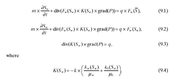
The initial and boundary conditions are

Equation (9.1) is the water fraction transport equation at the sources, and equation (9.2) is the water fraction transport equation in the domain. Equation (9.3) is the elliptic pressure equation. The solutions of this system involve water saturation, S_w (the fraction of water in the fluid flow), and pressure in the oil field, P. These equations include coefficients for the medium’s characteristics: the coefficient of porosity (m), the absolute permeability (k) and nonlinear relative phase permeabilities of oil (k_o(S_w)) and water (k_w(S_w)), the viscosities of oil (m₀) and water (m_w), the function of sources/sinks (q), critical and connected values of water saturation (S and S–) and the strongly nonlinear Bucley-Leverett function (F_w(S_w)).

The numerical solutions were sought in a domain with conditions of impermeability at the boundary (9.7). This domain was a subdomain of symmetry singled out from the unbounded oil field being simulated. The numerical algorithm was based on completely implicit methods of solving equations (9.1) through (9.3). That is, equations (9.1) and (9.2) were solved by the iterative secant method, while the (a–b)-iterative algorithm was employed to solve equation (9.3). The (a–b)-elliptic solver was an extension of the sweep method for the many-dimensional case. It did not need any a priori information about problem operators and was sufficiently general purpose. By this algorithm the solution being sought was obtained via eight auxiliary functions calculated iteratively. It was useful to include a relaxation parameter into the equations for some coefficients in order to reduce the number of (a–b)-iterations.

The standard seven-point (“honeycomb”) scheme of oil/water well disposition was simulated as shown in Figure 9.14. The computational domain was approximated by a uniform rectangular grid of 117 x 143 points.

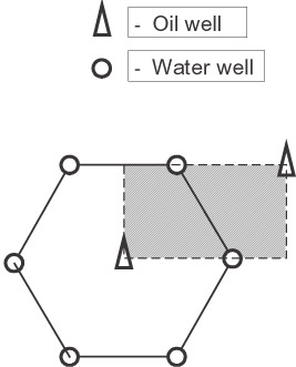
Figure 9.14: The seven-point “honeycomb” scheme of oil/water well disposition.

The parallel implementation of the algorithm for running on MPPs was based on computational domain partitioning. The domain was divided into equal subdomains in one direction along the Y-coordinate, with each subdomain being computed by a separate processor of an executing MPP.

That domain distribution was more successful in reducing the number of message-passing operations in the data parallel (a–b)-algorithm than the domain distributions along the X-coordinate or along both coordinates.

In each subdomain the system (9.1) through (9.3) was solved as follows: At every time level, the water saturation was found by solving equations (9.1) and (9.2) using the pressure values from the previous time level. Then, from the just obtained water saturation, a new pressure was calculated at the present time level by solving equation (9.3). This procedure was repeated at each subsequent time level.

The main difficulty of this parallel algorithm was estimation of the optimal relaxation parameter w for the (a–b)-solver because this parameter varies while dividing the computational domain into different quantities of equal subdomains. Employing a wrong parameter led to slow convergence or in some cases to nonconvergence of (a–b)-iterations. Numerous experiments allowed finding the optimal relaxation parameter for each number of subdomains.

The parallel algorithm above was implemented in Fortran 77 with PVM as a communication platform and demonstrated good scalability, speedups, and parallelization efficiency while running on the Parsytec PowerXplorer System—an MPP consisting of PowerPC 601 processors as computational nodes, and T800 transputers as communicational nodes (one T800 provides four bi-directional 20 Mbits/s communication links).

Table 9.2 presents some results of the experiments for one time level. The parallelization efficiency is defined as S_real/S_ideal x 100%, where S_real is the actual speedup achieved by the parallel oil extraction simulator on the parallel system, and S_ideal is the ideal speedup. S_ideal is calculated as the sum of speeds of processors of the executing parallel system divided by the speed of a base processor. All speedups are calculated relative to the original sequential oil extraction simulator running on the base processor. Note that the more powerful are the communication links and the less powerful are the processors, and the higher efficiency is achieved.

Table 9.2: Performance of the Fortran/PVM parallel oil extraction simulator on the Parsytec PowerXplorer System

Number of Processors	w	Number of Iterations	Time (s)	Real speedup	Efficiency
1	1.197	205	120	1	100%
2	1.2009	211	64	1.875	94%
4	1.208	214	38	3.158	79%
8	1.22175	226	26	4.615	58%

The parallel oil extraction simulator was thought to be part of a portable software system that would run on local networks of heterogeneous computers and provide a computerized working place of an oil extraction expert. Therefore a portable application efficiently solving the oil extraction problem on networks of computers was required.

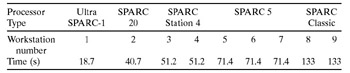
Our first step was to port the Fortran/PVM program to a local network of heterogeneous workstations based on 10 Mbits Ethernet. Our weakest workstation (SPARCclassic) executed the serial application a bit slower than PowerPC 601, while the most powerful one (UltraSPARC-1) executed it more than six times faster. In general, nine uniprocessor workstations were used, and Table 9.3 shows their relative speeds.

Table 9.3: Relative speeds of workstations

Workstation Number	Relative Speed
1	1150
2	575
3–4	460
5–7	325
8–9	170

Table 9.4 shows some results of execution of the Fortran/PVM program on different two-, four-, six-, and eight-workstation subnetworks of the network. For every subnetwork in this table the speedup is calculated relative to the running time of the serial program on the fastest workstation of the subnetwork. (The total running time of the serial oil extraction simulator while executing on different workstations can be found in Table 9.5.) The visible degradation of parallelization efficiency is explained as caused by the following: slower communication links, faster processors, and an unbalanced workload of the workstations.

Table 9.4: Performance of the Fortran/PVM parallel oil extraction simulator on subnetworks of workstations

Subnetwork (Workstation Number)	w	Number of Iterations	Time (s)	Ideal Speedup	Real Speedup	Efficiency
{2, 5}	1.2009	211	46	1.57	0.88	0.56
{5, 6}	1.2009	211	47	2.0	1.52	0.76
(2, 5–7}	1.208	214	36	2.7	1.13	0.42
{2–7}	1.21485	216	32	4.3	1.27	0.30
{2, 3, 5–8}	1.21485	216	47	3.8	0.87	0.23
{1–8}	1.22175	226	46	3.3	0.41	0.12

The first two are unavoidable, while the third can be avoided by slight modification of the parallel algorithm implemented by the Fortran/PVM program. That is, to provide the optimal load balancing, the computational domain should be decomposed into subdomains of nonequal sizes, proportional to relative speeds of participating processors. To be exact, the number of grid columns in each subdomain is the same, while the number of rows differs. This modified algorithm is hard to implement in portable form using PVM or MPI but can easily be implemented in mpC.

Regarding the relaxation parameter, it is reasonable to assume its optimal value to be a function of the number of grid rows, and to use its own relaxation parameter w= w(N_row) for each subdomain. While distributing the domain into different quantities of subdomains with equal numbers of grid rows, a sequence of optimal relaxation parameters can be found empirically. Now using the experimental data and piecewise linear interpolation, the optimal parameter w can be calculated for any N_row. Note in Table 9.6 that this approach gives a high convergence rate and good efficiency of the parallel (a–b)-solver with relaxation (see the numbers of iterations).

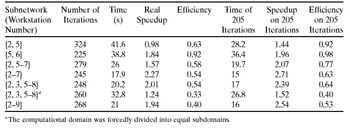
Table 9.6 shows experimental results of execution of the mpC application on the network of workstations. In the experiments the mpC programming environment used LAM MPI 6.0 as a communication platform. As can be seen, the mpC application demonstrates much higher efficiency in the heterogeneous environment than its PVM counterpart. To estimate the pure contribution of load balancing in the improvement of parallelization efficiency, we ran the mpC application on a subnetwork {2, 3, 5, 6, 7, 8} with a forcedly even domain decomposition, which resulted in the essential (more than 1.5 times) efficiency degradation (compare rows 5 and 6 in Table 9.6). Note that the mpC application only dealt with processor speeds and distributed data by taking into account only this aspect of heterogeneity.