The MDX SELECT Statement
The MDX SELECT statement is our means of extracting information from OLAP cubes. In the same way the T-SQL SELECT statement produces a result set from a relational database, the MDX SELECT statement produces a result set from a multidimensional database. The first major difference between the two statements is the T-SQL SELECT statement returns rows and columns, while the MDX SELECT statement returns a multidimensional result set that can contain rows and columns, but it also can contain things called pages, sections, and chapters. More on that in the "Additional Dimensions" section of this chapter.
The other difference between the T-SQL SELECT statement and the MDX SELECT statement is the MDX SELECT statement is easier. That may be hard for many of you relational database jockeys to believe, but it is true. Just work through this section and see if you don't agree.
When I say "work through this section," I mean it. This section is not labeled "Learn By Doing," but it might as well be. You can gain a better understanding if you read this in front of a running copy of the SQL Server Management Studio and try out each query as you go. By the time you're done, you'll agree this multidimensional analysis is no trouble at all.
The Basic MDX SELECT Statement
We begin with the most basic MDX SELECT statement and gradually acid complexity. When we are done, you should have a good understanding of the statement and be ready for almost any data analysis challenge. We begin with some brief instructions for opening an MDX Query window, so you can play along at home.
Opening a SQL Server Management Studio MDX Query Window
To open a SQL Server Management Studio MDX Query window pointing to the Max Min Manufacturing DM cube, do the following:
-
Open the SQL Server Management Studio.
-
Connect to the Analysis Services server hosting the MaxMinManufacturingDM database.
-
Expand the entry for this server in the Object Explorer window, and then expand the Databases Folder under this server.
-
Right-click the entry for the MaxMinManufacturingDM database and select New Query | MDX from the Context menu. The MDX Query window displays as shown in Figure 11-1.
-
The Cube drop-down list shows the cubes and perspectives available in the MaxMinManufacturingDM database. The database contains one cube, but it also contains two perspectives built on that cube. Select the Max Min Manufacturing DM cube, rather than one of the perspectives from the drop-down list.
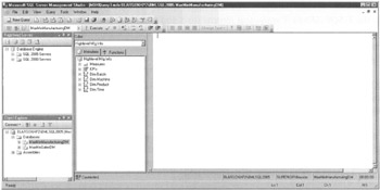
Figure 11-1: The SQL Server Management Studio with an MDX Query window
| Note | You can save your entries in the SQL Server Management Studio Query window by selecting the Save button in the toolbar or by selecting File | Save filename from the Main menu. |
The Very Basics
We begin with the most basic MDX SELECT statement possible:
SELECT FROM [Cube Name]
For example:
SELECT FROM [Max Min Manufacturing DM]
SELECT identifies this as a SELECT statement. The FROM clause identifies the cube or partition the information is selected from. This is known as the cube context for the SELECT statement. The result of this SELECT statement is shown in Figure 11-2.
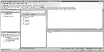
Figure 11-2: The most basic MDX SELECT statement
| Note | You can type SELECT FROM in the Query window, and then drag the name of the cube from the Metadata tab and drop it after the word "FROM" in the Query window. If you do this, make sure you unhighlight the cube name before executing the query. If any text is highlighted in the Query window, only that text is executed. This means you can have several query statements in the Query window at the same time and highlight the single query you want to execute. To execute the query, click the Execute button in the toolbar or press F5. |
When a SELECT statement executes, it creates a set of tuples, and then returns the value of one or more measures for each of those tuples. Remember, a tuple must contain one member from each dimension in the cube. This includes one of the measures in the cube that is considered to be part of the Measures dimension. A tuple from the Max Min Manufacturing DM cube includes the following dimensions:
(Dim Batch Hierarchy Member, Dim Machine Hierarchy Member, Dim Product Hierarchy Member, Dim Time Hierarchy Member, Measures Member)
In our basic MDX SELECT statement, we are not specifying the members of any dimensions to be included in the result. As we learned in Chapter 10, when a member is not explicitly specified for a dimension, the default member is used. Therefore, our query must be using the default members for all of the dimensions, including the Measures dimension, to get the result.
The tuple that defines our result is
([Dim Batch].[Dim Batch].DefaultMember, [Dim Machine].[Material Hierarchy].DefaultMember, [Dim Product].[Product Hierarchy].DefaultMember, [Dim Time].[Time Hierarchy].DefaultMember, [Measures].DefaultMember)
The default member for most of the dimensions is All. Recall we set the default member for the Time dimension to 2005. The default member for the Measures dimension is the first measure we defined, namely the Accepted Products measure. So, the equivalent tuple is
([Dim Batch].[Dim Batch].[All], [Dim Machine].[Material Hierarchy].[All], [Dim Product].[Product Hierarchy].[All], [Dim Time].[Time Hierarchy].[2005], [Measures].[Accepted Products])
By executing our basic MDX SELECT statement, we learned that for all batches, all materials, and all products for the year 2005, a total of 3,418,942 products were accepted.
Query Dimensions
As you might expect, we need to be able to specify members other than the default members in our MDX SELECT statements for those statements to be of much interest. We do this by including query dimensions. An MDX SELECT statement with one query dimension has the following format:
SELECT {set of dimension members} ON COLUMNS FROM [Cube Name] For example:
SELECT {[Guiding Lights], [Mythic World], [Warriors of Yore], [Woodland Creatures]} ON COLUMNS FROM [Max Min Manufacturing DM] Remember, a set is enclosed in curly brackets ( { } ). The results of this statement are shown in Figure 11-3.
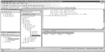
Figure 11-3: An MDX SELECT statement with a query dimension
| Note | As with the cube name, you can locate the dimension members in the Metadata tab, and then drag-and drop them into the query. Spaces, tabs, and new lines can be used interchangeably in MDX queries. The new lines are used in the code listing and figures to display the SELECT statements conveniently in the space allowed. Also, the query editor does syntax checking via Intellisense to give you cues if your query is not in proper form. |
If you are paying attention, you realize we can save ourselves some typing and enter this query as follows:
SELECT [Dim Product Type].Members ON COLUMNS FROM [Max Min Manufacturing DM]
When a set of members is specified in this manner, the curly brackets are optional.
Figure 11-4 illustrates how the COLUMNS query dimension is used to create the result set of the SELECT statement. A tuple is created using each member of the COLUMNS query dimension. A value is then retrieved for the member of the Measures dimension in each tuple.
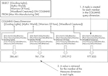
Figure 11-4: Creating a result with a COLUMNS query dimension
Let's add a second query dimension to our MDX SELECT statement. With two query dimensions, the MDX SELECT statement has the following format:
SELECT {set of dimension members} ON COLUMNS, {set of dimension members} ON ROWS FROM [Cube Name] For example:
SELECT [Product Type].Members ON COLUMNS, [Year].Members ON ROWS FROM [Max Min Manufacturing DM]
The results of this statement are shown in Figure 11-5.
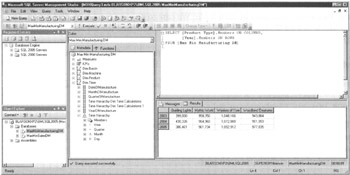
Figure 11-5: An MDX SELECT statement with two query dimensions
Figure 11-6 illustrates how the COLUMNS query dimension and the ROWS query dimension are used to create the result set of the SELECT statement. A tuple is created combining each member of the COLUMNS query dimension with each member of the ROWS query dimension. A value is then retrieved for the member of the Measures dimension in each tuple. We can go beyond two query dimensions in an MDX SELECT statement, but we save that discussion for the section "Additional Dimensions."
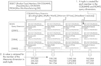
Figure 11-6: Creating a result with two query dimensions
Because Measures is considered another dimension of our cube, we can use a set of dimension members for a query dimension. For example:
SELECT {[Measures].[Accepted Products], [Measures].[Total Products]} ON COLUMNS, [Year).Members ON ROWS FROM [Max Min Manufacturing DM] This MDX SELECT statement uses a set containing the Accepted Products measure and the Total Products calculated member for the COLUMNS query dimension. The result is shown in Figure 11-7. We end up with the total of all accepted products and the total of all products for each year.
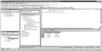
Figure 11-7: Measures dimension members in the COLUMNS query dimension
Slicer Dimension
Using members of the Measures dimension in a query dimension is one way to view different measures in the result set. Using a slicer dimension is another. When using a slicer dimension, the MDX SELECT statement has the following format:
SELECT {set of dimension members} ON COLUMNS, {set of dimension members} ON ROWS FROM [Cube Name] WHERE [Measures dimension member] For example:
SELECT [Product Type].Members ON COLUMNS, [Year].Members ON ROWS FROM [Max Min Manufacturing DM] WHERE [Measures].[Total Products]
The results of this statement are shown in Figure 11-8. Remember, the default Measure is Accepted Products. Now in this result set, we get the total products for each product type for each year.
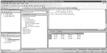
Figure 11-8: An MDX SELECT statement with a slicer dimension
In addition to specifying the measure used in the result set, we can use the slicer dimension to do a bit more. We can specify dimension members to use in place of our default members for dimensions not included in the query dimensions. The format for this type of MDX SELECT statement is
SELECT {set of dimension members} ON COLUMNS, {set of dimension members} ON ROWS FROM [Cube Name] WHERE ([Measures dimension member], [dimension member]) The WHERE clause now contains a tuple, rather than a single Measures dimension member. This tuple can include as many dimension members as you like. The rule is this: a dimension can only appear in one place in the MDX SELECT statement, either on one of the query dimensions or in the slicer dimension.
This sounds confusing, but an example clears things up. Suppose we want to see the total products for our product types for each of the years in the cube, but we only want to see those numbers as they pertain to the Maximum Miniatures plant in Fridley (Plant #3). We can use the following MDX SELECT statement to get this information:
SELECT [Product Type].Members ON COLUMNS, [Year].Members ON ROWS FROM [Max Min Manufacturing DM] WHERE ([Measures].[Total Products], [Dim Plant].&[3])
The result of this query is shown in Figure 11-9.
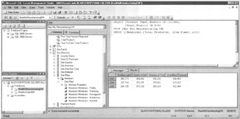
Figure 11-9: An MDX SELECT statement with a tuple in the slicer dimension
Figure 11-10 illustrates how the tuple in the slicer dimension affects the result set. Each member of the COLUMNS query dimension is combined with each member of the ROWS query dimension. These combinations are then combined with the members of the slicer dimension tuple. The default member is used for any dimension not represented in the COLUMNS query dimension, the ROWS query dimension, or the sheer dimension tuple.
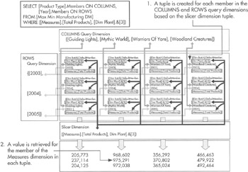
Figure 11-10: Creating a result with a slicer tuple
Filtering with the FILTER Function
Many times, as we are creating MDX SELECT statements, the set of members we want to see on a dimension is dependent on the content of the data. For example, the production manager at Maximum Miniatures may want to see the number of accepted products produced for those products that had an increase in their backorder amounts during the month. The production manager does not want to see all of the products in the dimension, only those with a higher amount on backorder. It is not possible to manually type a set of products to satisfy this query from month to month. A product that may have an increasing backorder from May to June may not be in that same state from June to July. It all depends on the data.
Fortunately, the FILTER function, which is an MDX function, lets us determine the content of a set using a condition expression.
The FILTER function starts with a set of members as a parameter. Then it removes members from the set that do not satisfy the condition expression. Let's see if we can come up with a FILTER condition that can satisfy the production manager. We can compare the backorder amounts for November 2005 and December 2005.
If you switch to the Functions tab, you find the FILTER function in the Set folder because it returns a set. Drag the FILTER function and drop it on the Query window to use it as the content of one of the query dimensions. You see the following:
FILTER( «Set», «Search Condition» )
The syntax tells us we need to supply the FILTER function with two parameters: a set and a search condition.
The set should be all members of the Product dimension at the product level. The FILTER function then removes those products that do not meet the search condition. The expression [Product] provides a list of all products.
For the search condition, we use an expression comparing two values with a Boolean operator. The values we are creating come from two tuples. The first tuple is composed of the December 2005 member of the MonthofManufacture hierarchy along with the Accepted Products measure. The second tuple is composed of the November 2005 member of the MonthofManufacture hierarchy along with the Accepted Products measure.
These two tuples are evaluated by including each member of the set of Products (the first parameter of the function) one at a time. The function evaluates
([Product].[American GI], [MonthOfManufacture].[200512] , [Measures].[Number On Backorder]) < ([Product].[American GI], [MonthOfManufacture].[200511] , [Measures].[Number On Backorder])
and then it evaluates
([Product].[Bear and Cub], [MonthOfManufacture].[200512], [Measures].[Number On Backorder]) < ([Product].[Bear and Cub], [MonthOfManufacture].[200511], [Measures].[Number On Backorder])
Any members of the set of Products that result in an expression evaluating to true are included in the set returned as the FILTER function's result. The result is then used by the SELECT statement to create columns. The MDX SELECT statement and its result are shown in Figure 11-11.
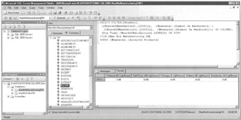
Figure 11-11: An MDX SELECT statement using the FILTER function
Note, a number of products show "(null)" for the number of accepted products in December 2005. This occurs because this product was not manufactured in December 2005. No data exists to report for this measure in this timeframe, which probably explains why the number of backorders increased for these products!
Additional Tools for Querying
We have now covered the basics of the MDX SELECT statement. You've seen how to quickly assemble dimensions, hierarchies, and measures to analyze the cube data and discover Business Intelligence (BI). However, a few more tools can help take the query process one step further.
The WITH Statement
In the previous section, we used the FILTER function to create the desired set for one of our query dimensions. But, there may be times when the desired set cannot be defined by an expression in a FILTER function. Perhaps we want to look at the production of American WWII figures. There is nothing that lets us create this set using a filter (at least not a straightforward filter). We need to build this set manually.
Rather than putting this manually created set in the MDX SELECT statement itself, we can use the WITH statement to define a named set. Once the named set is defined, it can be used in the MDX SELECT statement. The format for a WITH statement creating a named set is
WITH SET [named set name] AS '{set definition}' Here is the WITH statement and an MDX SELECT statement that uses it:
WITH SET [American WWII Figures] AS '{[American GI], [US Army Pilot], [US Navy Gunner"s Mate]}' SELECT {[American WWII Figures]} ON COLUMNS, [Year].Members ON ROWS FROM [Max Min Manufacturing DM] WHERE [Measures].[Total Products] The results are shown in Figure 11-12.
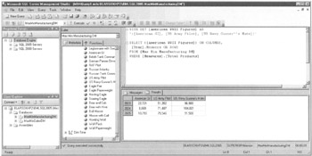
Figure 11-12: An MDX SELECT statement using a named set
| Note | We must enclose the string defining the set in single quotes. This poses a bit of a challenge because one of the member names contains a single quote, or more accurately, an apostrophe. To make this work, we need to double the single quote contained within the string. |
The main advantage of the named set is to keep your MDX SELECT statements neat, easily understandable, and self-documenting. The named set is also reusable. As we saw in Figure 11-3, even a simple query can look rather complex when a large set is specified right in one of the query dimensions. Named sets provide a way to avoid these complex statements by splitting things up.
We can also use the WITH statement to define temporary calculated members. These can be members of one of our dimensional hierarchies or members of the Measures dimension. The format for a WITH statement that defines a temporary calculated member is
WITH MEMBER [parent member].[calculated member name] AS '{member definition}' Let's expand on our American WWII Figures set and create calculated members that create rollups for each nationality in the WWII product subtype.
Here is the code:
WITH MEMBER [World War II].[American Figures] AS '[American GI]+[US Army Pilot]+[US Navy Gunner"s Mate]' MEMBER [World War II].[British Figures] AS '[British Tank Commander]+[RAF Pilot]' MEMBER [World War II].[Russian Figures] AS '[Russian Infantry]+[Russian Tank Commander]' MEMBER [World War II].[German Figures] AS '[German Panzer Driver]' SELECT {[American Figures], [British Figures], [Russian Figures], [German Figures]} ON COLUMNS, [Year].Members ON ROWS FROM [Max Min Manufacturing DM] WHERE [Measures].[Total Products] The results are shown in Figure 11-13.
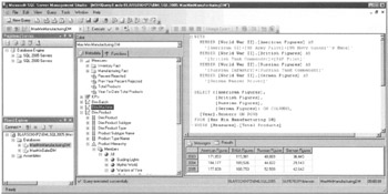
Figure 11-13: An MDX SELECT statement using temporary calculated members
The difference between the named set and the calculated member can seem a bit subtle at first glance. The named set is just that—a set of individual members. When we used the set in Figure 11-12, each of the individual members appeared in the result set.
Each calculated member is a new individual member that is composed of the aggregation of information from other members. When the calculated members are used in Figure 11-13, only the newly defined calculated members, not their constituent parts, appear in the result set.
While we are at it, let's define a temporary member of the Measures dimension. Suppose we want to know what percentage of total production our members of the product hierarchy accounted for. We can define a temporary calculated member of the Measures dimension and use it as follows:
WITH MEMBER [Measures].[Percent Of Parent] AS 'CStr(ROUND(([Product Hierarchy].CurrentMember, [Measures].[Total Products])*100/ ([Product Hierarchy].CurrentMember.Parent, [Measures].[Total Products]},2))+"%"' SELECT {[Product Type].Members} ON COLUMNS, [Year].Members ON ROWS FROM [Max Min Manufacturing DM] WHERE [Measures].[Percent Of Parent] The expression used to define the temporary calculated member is somewhat complex: it consists of two tuples. The first tuple:
([Product Hierarchy].CurrentMember, [Measures].[Total Products])
returns the value of the total products measure for the current member of the product dimension. The second tuple:
([Product Hierarchy].CurrentMember.Parent, [Measures].[Total Products])
returns the value of the total products measure for the parent of the current member of the product dimension. We multiply the total products value from the current member by 100, and then divide it by the total products value from the parent member. The resulting decimal number is rounded to two decimal places and converted to a string. Finally, we concatenate the percent sign on the end. There you have it.
The results are shown in Figure 11-14.
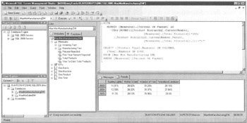
Figure 11-14: An MDX SELECT statement using a temporary calculated member of the Measures dimension
| Note | If you are working through these examples on your computer, you will notice the color coding on the Query window gets a bit confused with the new lines in the middle of the string defining the calculated member. Despite this, the query executes without a problem. |
CROSSJOIN
Up to this point, our MDX SELECT statements have been limited to one dimension on each query dimension. Given that they are called query dimensions, it does make sense that would be the case. However, at times, we would like to break what seems an obvious correlation and put two dimensions on a single query dimension. Fortunately, MDX provides a way to do just that. (Of course it does; otherwise, I wouldn't have brought it up!)
We use the CROSSJOIN function to combine sets from two dimensions into a single joined set. This joined set can then be placed on a query dimension. If you are familiar with the cross join in T-SQL, you have a pretty good idea how this is going to work. Our new set is going to be made out of tuples, which combine every member of one set with every member of the other set.
If you switch to the Functions tab, you find the CROSSJOIN function in the Set folder because it returns a set. Drag the CROSSJOIN function and drop it on the Query window. You see the following:
CROSSJOIN( <<Set1>>, <<Set2>> )
The syntax tells us we need to supply the CROSSJOIN function with two parameters, both sets. Let's look at an example.
Suppose we want to see the total products by product type by plant by year. We have three dimensions to work with. Here is what it looks like using the CROSSJOIN function:
SELECT CROSSJOIN({[Product Type].Members}, {[Plant].Members}) ON COLUMNS, ([Year].Members} ON ROWS FROM [Max Min Manufacturing DM] WHERE [Measures].[Total Products] In this query, we are taking all of the members of the product type hierarchy and cross joining them to all of the members in the plant hierarchy. With four product types and five plants, we end up with 20 tuples in the cross-joined set and 20 columns in the result set. The result is shown in Figure 11-15.
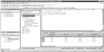
Figure 11-15: An MDX SELECT statement using the CROSSJOIN function
NON EMPTY and NON EMPTY CROSSJOIN
If you look at the result set in Figure 11-15, you see a number of (null) entries. This indicates a particular product type was not manufactured at a particular plant during that year. For example, there have never been any products from the Guiding Lights product type manufactured at the Hamburg plant. Let's make our result set easier to analyze by eliminating columns with null values in every row. We do that by adding the NON EMPTY keyword to the MDX SELECT statement.
The NON EMPTY keyword can be placed in front of the CROSSJOIN or in front of the set in any of the query dimensions. It eliminates any members that do not have corresponding values in the Measures dimension. The NON EMPTY keyword is not limited to sets derived from CROSSJOIN functions. It can be added to a query dimension anytime there are null values we would like to remove from the result set.
With the NON EMPTY keyword included, our query looks like this:
SELECT NON EMPTY CROSSJOIN({[Product Type].Members}, {[Plant].Members}) ON COLUMNS, {[Year}.Members} ON ROWS FROM [Max Min Manufacturing DM} WHERE [Measures].[Total Products] The results, with the empty columns removed, are shown in Figure 11-16.
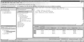
Figure 11-16: An MDX SELECT statement using the NON EMPTY keyword
TOPCOUNT/BOTTOMCOUNT
Often during analysis, we want to see the highest or the lowest values for a given measure. Of course, we can manually scan the rows and columns of numbers to make this determination. However, the more information we need to sift through, the more this becomes an arduous and error-prone task. Instead, we should have our MDX SELECT query do this analysis for us.
This is where the TOPCOUNT and BOTTOMCOUNT functions come in. These functions return the select set of the members with the highest or lowest values for a specified measure. The TOPCOUNT and BOTTOMCOUNT functions are found in the Set folder because they each return a set. Drag the TOPCOUNT function and drop it on the Query window. You see the following:
TOPCOUNT( <<set>>, <<Count>>[, <<Numeric Expression>>] )
The first parameter is the set we are to select from. The second parameter is the number of members to include in our result set. The third parameter is the numeric expression, usually a measure, which is used to rank the set members before taking the requested number of members off the top. The syntax of the BOTTOMCOUNT function is identical to that of the TOPCOUNT. The only difference, of course, is the BOTTOMCOUNT is pulling from the bottom of the ranking rather than the top.
Let's begin by looking for the five products we have manufactured the most in 2005. To accomplish this, we use the TOPCOUNT function in the following query:
SELECT TOPCOUNT([Product].Members, 5, [Measures].[Total Products]) ON COLUMNS FROM [Max Min Manufacturing DM]
The results are shown in Figure 11-17. Note, we now only have five products in the result set, but the products are in their ranking order.
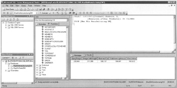
Figure 11-17: An MDX SELECT statement using the TOPCOUNT function
To find the three machines that have manufactured the least amount of product in 2005, we can use the following query:
SELECT BOTTOMCOUNT([Machine].Members, 3, [Measures].[Total Products]) ON COLUMNS FROM [Max Min Manufacturing DM]
The results are shown in Figure 11-18.
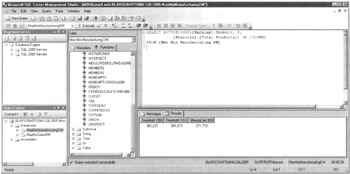
Figure 11-18: An MDX SELECT statement using the BOTTOMCOUNT function
Remember, the TOPCOUNT and BOTTOMCOUNT functions simply create a set to use in one of the query dimensions. Let's look at another example to illustrate this point:
SELECT TOPCOUNT([Product].Members, 5, [Measures].[Total Products]) ON COLUMNS, {[Year].[2004]} ON ROWS FROM [Max Min Manufacturing DM] The results are shown in Figure 11-19.
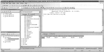
Figure 11-19: An MDX SELECT statement using the TOP COUNT function along with a ROWS query dimension
At first, a problem seems to exist with the result set shown in Figure 11-19. The products do not appear in the proper rank order. Maximum Miniatures made more Bear and Cub than Dragon with Knight, yet Dragon with Knight is second in the result set and Bear and Cub is third. We need to look at exactly what our MDX SELECT statement is doing.
The TOPCOUNT function executes first to create the set for the COLUMNS query dimension. Because we have not specified a member of the Time dimension, the function uses the default member of 2005. It finds the five products with the largest production in 2005. Using this set of five products for the COLUMNS query dimension, the SELECT statement combines it with the 2004 member from the ROWS query dimension to get the total production for our five products in 2004. Dragon with Knight production may have exceeded Bear and Cub production in 2005, but it did not in 2004. As with most computer code, you usually get exactly what you ask for. The trick is asking for the correct thing!
Aggregates
We have looked at aggregate functions with respect to the rollup done for hierarchy members in the cube. MDX also offers aggregation functions that may be used for creating calculations in MDX SELECT statements. We examine two of these functions here.
First, the SUM function adds the values of a numeric expression for all of the members in a set. The format of the SUM function is
SUM( <<Set>>[, <<Numeric Expression>>] )
Second, the COUNT function counts the number of items in a set. The COUNT function has the following format:
COUNT( <<Set>>[, EXCLUDEEMPTY | INCLUDEEMPTY] )
The optional second parameter to the COUNT function determines whether empty cells are counted.
Let's use these two aggregate functions to calculate the average amount produced per month for each product. We use the following query:
WITH MEMBER [Measures].[Avg per Month] AS 'ROUND(Sum(Descendants([Time Hierarchy].CurrentMember, [Day]), [Measures].[Total Products]) / Count(Descendants([Time Hierarchy].CurrentMember, [Day])),0)' SELECT [Year].Members ON COLUMNS, [Product Type].Members ON ROWS FROM [Max Min Manufacturing DM] WHERE [Measures].[Avg per Month]
In our temporary calculated member, we first find the descendants of the current time hierarchy member at the day level. We then take the SUM of the Total Products measure to determine the number produced for this time period. We also take the COUNT of the number of time days in the current time hierarchy member. We can then divide the sum of the total products produced by the sum of the number of days in the time period to get the average. Add a Round function to get rid of the fraction amount and we are done. The results are shown in Figure 11-20.
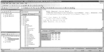
Figure 11-20: An MDX SELECT statement using SUM and COUNT aggregates
| Note | MDX also includes a DISTINCTCOUNT function that has the same structure and function as the COUNT function. The only difference is the DISTINCTCOUNT function counts multiple occurrences of a member in the set only once. |
Additional Dimensions
To this point, we have worked only with the COLUMNS and ROWS query dimensions. We did hint that more dimensions were possible. Indeed, though it is hard for our brains to visualize in more than three dimensions. Analysis Services can provide many more.
Pages, Sections, and Chapters
Five named query dimensions are supported by the MDX SELECT statement. They are
-
COLUMNS
-
ROWS
-
PAGES
-
SECTIONS
-
CHAPTERS
These query dimensions must be used in the order they are presented here. You cannot have a ROWS query dimension in your MDX SELECT statement unless a COLUMNS query dimension is also present. You cannot have a PAGES query dimension in your MDX SELECT statement unless ROWS and COLUMNS query dimensions are also present, and so on.
AXIS(n)
The MDX SELECT statement supports a number of query dimensions beyond the live named query dimensions. Indeed, it is possible to define up to 128 query dimensions. Once we move beyond live, we refer to the query dimensions as AXIS(n). In fact, we can use AXIS(0) in place of COLUMNS, AXIS(1) in place of ROWS, like so:
SELECT [Product Type].Members ON AXIS(0), [Year].Members ON AXIS(1) FROM [Max Min Manufacturing DM] WHERE [Measures].[Total Products]
The results are shown in Figure 11-21.
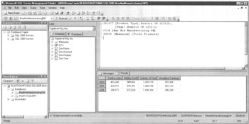
Figure 11-21: An MDX SELECT statement using AXIS(0) and AXIS(1)
Unfortunately, the Query window in the SQL Server Management Studio does not display more than two query dimensions. When we try, we receive an error message as shown in Figure 11-22. This is an error from the front-end Query window, not from the Analysis Services server. Other front-end tools allow for more dimensions in our queries.
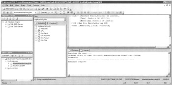
Figure 11-22: A front-end Query window error when trying to use three query dimensions
EAN: 2147483647
Pages: 112