9.4. Robust Expressions and Predicates
| | ||
| | ||
| | ||
9.4. Robust Expressions and Predicates
In this section, we will present useful expressions and predicates that occur very often in geometric algorithms. There are many different ways for evaluating a geometric expression or predicate. A careful analysis often leads to relatively stable results. In Section 9.3.1, we saw that without a guard digit, the relative error obtained when subtracting nearby numbers can be very large. We should take this into account. Appropriate representations of geometric expressions are useful for almost all arithmetic strategies considered in Section 9.3.
We consider two simple examples stemming from [Shewchuk 99] and [Goldberg 91]. Both examples depend on floating-point roundoff errors (see Section 9.3.1). We will see that it is worth thinking about a robust representation of arithmetic expressions. A formula can sometimes be rearranged in order to eliminate catastrophic cancellation. The third example stemming from [Goldberg 91] shows a formal justification of the rearrangement, due to backward-error analysis. The given rearrangement ideas can be justified formally . Later in Section 9.4.2, we will summarize a list of useful robust expressions. Many expressions will be represented by the sign of determinants. The evaluation of determinants is incorporated into standard computer algebra systems. For an efficient and robust evaluation of the sign of determinants , see also [Clarkson 92], [Kaltofen and Villard 04] or [Avnaim et al. 97].
9.4.1. Examples of Formula Rearrangement
The area of a simple polygon. The area of a simple polygon in two dimensions can be computed by a simple formula. Let p 1 , p 2 , p 3 , , p n denote the counterclockwise sequence of the vertices of a polygon P . The signed area of the polygon is
| (9.5) | 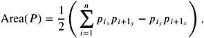 |
where ![]() and p n + 1 := p 1 . Area ( P ) is positive if P is given in counter-clockwise order. If P is given in clockwise order, Area ( P ) is negative. This can be easily shown by induction on the number of vertices.
and p n + 1 := p 1 . Area ( P ) is positive if P is given in counter-clockwise order. If P is given in clockwise order, Area ( P ) is negative. This can be easily shown by induction on the number of vertices.
The robustness of Equation (9.5) depends on the relationship of the absolute value of the coordinates to the area of the polygon. If the area is relatively small and the absolute value of the coordinates are relatively high, i.e., the distance to the origin is relatively high, then roundoff errors in floating-point operations may lead to inaccurate results. Therefore, we translate the polygon near to the origin by using the points ![]() . It is easy to see that
. It is easy to see that
| (9.6) | 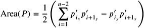 |
holds. This simply follows from the fact that the area is invariant due to a translation of the polygon. The last formula is much more robust than Equation (9.5), since we do not have severe cancellations .
For example, let us consider the rectangle P given by p 1 = (301, 300), p 2 = (301 , 301), p 3 = (300, 301), and p 4 = (300, 300); see Figure 9.17.

Figure 9.17: Computing the area of a rectangle P.
Using Equation (9.5) for = 10 and p = 4, we obtain the incorrect results 301 ![]() 301 = 90600 and 301
301 = 90600 and 301 ![]() 300 = 90300 due to the round-to- nearest rule. This gives
300 = 90300 due to the round-to- nearest rule. This gives
whereas using ![]() , P is given by
, P is given by ![]() ,
, ![]() ,
, ![]() , and
, and ![]() . Now, for P , the exact result is calculated by
. Now, for P , the exact result is calculated by
Keep in mind that normally there is a speed trade-off we have to pay for robustness. Obviously in Equation (9.6) we need more floating-point operations than in Equation (9.5).
Translation near to the origin is a robustness paradigm, and we will use this principle especially for geometric predicates and constructors; see Section 9.4.2.
The solutions of a quadratic equation. The solution of a quadratic equation
| (9.7) | |
is given by
| (9.8) | 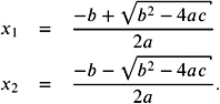 |
The expression b 2 ˆ 4 ac could be the result of a floating-point subtraction of two floating-point multiplications. If b 2 and 4 ac are rounded to nearest, they are accurate within 1/2 ulp. Now subtraction may cause many of the accurate digits to disappear. Therefore, the result of the difference may have an error of many ulps.
For example, for p = 3 and = 10, let b = 3 . 34, a = 1 . 22, and c = 2 . 28. The exact value of b 2 ˆ 4 ac is 0 . 0292, whereas b ![]() b = 11 . 2, 4
b = 11 . 2, 4 ![]() a
a ![]() c = 11 . 1, and 11 . 2
c = 11 . 1, and 11 . 2 ![]() 11 . 1 results exactly in 0 . 1. This means that the overall error is in 70 . 8 ulps.
11 . 1 results exactly in 0 . 1. This means that the overall error is in 70 . 8 ulps.
If b 2 ‰ˆ 4 ac , cancellation is not a problem in Equation (9.8), since b will dominate the denominator. If b 2 ‰ 4 ac , then b 2 ˆ 4 ac does not cause cancellations, but ![]() ‰ˆ b is critical. One of the formulas of Equation (9.8) may produce the elimination of accurate digits. Therefore, we multiply the numerator and the denominator by ˆ b ˆ
‰ˆ b is critical. One of the formulas of Equation (9.8) may produce the elimination of accurate digits. Therefore, we multiply the numerator and the denominator by ˆ b ˆ ![]() and ˆ b +
and ˆ b + ![]() , respectively, and we obtain
, respectively, and we obtain
| (9.9) | 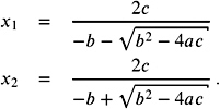 |
Let b 2 ‰ 4 ac . We use the following rule: if b > 0, compute x 2 by Equation (9.8) and x 1 by Equation (9.9); if b < 0, compute x 1 by Equation (9.8) and x 2 by Equation (9.9).
The expression x 2 ˆ y 2 . Although one might expect that an additional subtraction (addition) will cause a cancellation of accurate digits, we normally prefer the righthand side of
| (9.10) | |
By Theorem 9.10, the subtraction (addition) of two values without rounding errors (here x and y ) will have a small relative error. Multiplication of two quantities with a small relative error results in a product of small relative error.
If x ‰ y or y ‰ x , we will prefer the left-hand side of Equation (9.10). We do not have accurate digit eliminations here. Additionally, the rounding error of the smaller value ( x 2 or y 2 ) does not affect the final subtraction. In comparison to ( x ˆ y )( x + y ), we have to deal only with two rounding errors instead of three (for ( x ˆ y ), ( x + y ), and for the product ( x ˆ y )( x + y )).
We will give a formal justification for the given result. The standard technique for a theoretical analysis is called backward-error analysis . We can assume that subtraction, addition, and multiplication are performed as required in the standard; see Equation (9.2).
Therefore, we have to compare the relative error of
| (9.11) | |
to the relative error of
| (9.12) | 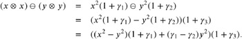 |
The relative error of Equation (9.11) is
which is equal to 1 + 2 + 3 + 1 2 + 2 3 + 1 3 + 1 2 3 ‰ 3( ![]() +
+ ![]() 2 ) +
2 ) + ![]() 3 .
3 .
The relative error of Equation (9.12) is
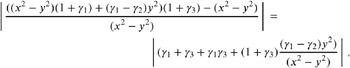
which gives a problem if x and y are nearby. In this case, ( 1 ˆ 2 ) y 2 can be as large as ( x 2 ˆ y 2 ), and the relative error appears to be approximately bigger than (1 + 3 ). If x ‰ y holds, the term
is negligible, and we obtain a result almost independent from 2 and approximately smaller than 2 ![]() +
+ ![]() 2 . Analogously, we can argue for y ‰ x .
2 . Analogously, we can argue for y ‰ x .
9.4.2. A Summary of Robust Expressions
The area of a triangle. Assume that the length of the sides a , b , and c of triangle T are given. Note that in Section 9.4.1 the coordinates of the points were given. Then the area of T , Area( T ), may be computed by
| (9.13) | |
where
Without loss of generality, we can assume that a ‰ b ‰ c . Otherwise, we rename the identifiers. Similar to the considerations in the previous section, Equation (9.13) has severe cancellations if a ‰ˆ b + c holds, i. e., the triangle is extremely flat. In this case, we have s ‰ˆ a , and the term ( s ˆ a ) subtracts two nearby quantities while s may have rounding errors. In this case, we might lose many accurate digits. We rearrange Equation (9.13) as follows
| (9.14) | |
Equation (9.14) is much more accurate because it avoids severe cancellation at hand. It can be shown that the four factors are non-critical. For example, a ![]() b is computed exactly with a guard digit. By backward-error analysis, the following result can be proven; see [Goldberg 91].
b is computed exactly with a guard digit. By backward-error analysis, the following result can be proven; see [Goldberg 91].
Theorem 9.29. If the machine epsilon ![]() is not greater than 0.005, then Equation (9.14) is correct within a relative error not greater than 11
is not greater than 0.005, then Equation (9.14) is correct within a relative error not greater than 11 ![]() .
.
If the triangle is given by the three endpoints, we can use the oriented area formula, detailed below.
In the following, we turn over to a list of robust geometric predicates and constructors.
Orientation test in 2D. The orientation test is used in many geometric algorithms. Given three points p , q , and r in the plane, we want to find out whether chain( p, q, r ) makes a left turn or right turn running from p over q to r . In the mathematical sense, a counterclockwise (left) turn is meant to be positive. One may think also of the orientation of the quadrants of a coordinate system in 2D.
The orientation test has various applications. For example, if we would like know whether two line segments l 1 = ( p 1 , q 1 ) and l 2 = ( p 2 , q 2 ) will have an intersection, we test whether the endpoints of l 2 do not lie on one side of l 1 and vice versa. Therefore, we have to check that chain( p 1 , q 1 , p 2 ) and chain( p 1 , q 1 , q 2 ), as well as chain( p 2 , q 2 , p 1 ) and chain( p 2 , q 2 , q 1 ), do not have the same orientation.
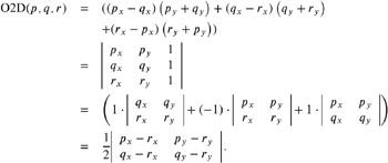
The semantic of the orientation test in 2D (O2D) is as follows:
For the computation of the orientation test of p , q , and r , we make use of the signed area of the parallelogram spanned by p , q , and r or equivalently determined by the vectors ![]() and
and ![]() .
.
The last expression is more accurate than the former ones. We simply translate all points by ˆ r , so that the relation between the absolute value of the points and the correlation to each other avoids severe cancellations; see also Section 9.4.1.
We are mainly interested in the sign of O2D; therefore, O2D sometimes is defined as a Boolean predicate, i.e., O2D( p, q, r ) = TRUE if chain( p, q, r ) is in counterclockwise order and so on; see also Section 9.6.
As a consequence for the signed area of the triangle of p , q , and r , we have
i. e., half of the area of the parallelogram.
Area of a triangle in 3D. For two vectors ![]() = ( u x , u y , u z ) and
= ( u x , u y , u z ) and ![]() = ( w x , w y , w z ) in
= ( w x , w y , w z ) in ![]() 3 , the vector cross product is defined by
3 , the vector cross product is defined by
which sometimes is denoted by the determinant
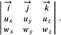
where ![]() = (1 , , 0),
= (1 , , 0), ![]() = (0 , 1 , 0), and
= (0 , 1 , 0), and ![]() = (0 , , 1).
= (0 , , 1).
Let p , q , and r define a triangle d in 3D. The vector cross product v = ![]() —
— ![]() results in a vector
results in a vector ![]() orthogonal to d , and the area of the triangle in 3 D is given by half of the length of
orthogonal to d , and the area of the triangle in 3 D is given by half of the length of ![]() .
.
For p = ( p x , p y , p z ), let p xy denote ( p x , p y ) in the xy -plane. p xz and p yz are defined analogously. Obviously, the x -coordinate of v x of v is given by
Analogously, we have v y = O2D( p zx , q zx , r zx ) and v z = O2D( p xy ,q xy , r xy ). Altogether, the area of the triangle d in 3D is given by
Note that the consideration of the cross product fits exactly to the 2D case. We can extend the 2D vectors ![]() and
and ![]() to the 3D setting
to the 3D setting ![]() = ( p x ˆ r x , p y ˆ r y , 0) and
= ( p x ˆ r x , p y ˆ r y , 0) and ![]() = ( q x ˆ r x , q y ˆ r y , 0). The vector cross product results in
= ( q x ˆ r x , q y ˆ r y , 0). The vector cross product results in
and the length of this vector equals O2D( p, q, r ).
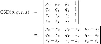
Orientation test in 3D. In 3D, a similar test can be applied. Having four points p , q , r , and s in 3D, we want to find out whether s lies below or beyond a 2D plane E spanned by the p , q , and r . Obviously, we have to specify what below and above mean exactly, which can be done by fixing the orientation of E . If we see the points p , q , and r from s in a counterclockwise order, the plane is meant to be seen from above , which gives a negative value. The orientation test O3D( p, q, r, s ) is positive if s lies below the oriented plane.
The semantic of the orientation test in 3D (O3D) is as follows:
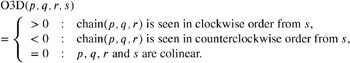
There is a nice thumb rule for the test. Take your left hand and try to point with slightly curled fingers to the points p , q , and r in a circular and clockwise manner, starting with the leftmost finger, thus describing an oriented plane. If your (hopefully shorter) thumb points to s , O3D returns a positive value.
Geometrically speaking and in analogy to O2D, the expression O3D( p, q, r, s ) is the signed volume of the parallelepiped determined by the vectors ![]() ,
, ![]() , and
, and ![]() . It is positive if the points are in position as described earlier; see also Figure 9.18.
. It is positive if the points are in position as described earlier; see also Figure 9.18.
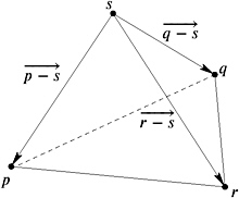
Figure 9.18: The chain p, q, and r is clockwise if we look from the top. The vertex s lies below the oriented plane and O3D(p, q, r, s) is positive.
Altogether, it suffices to evaluate the following determinant.
Due to [Shewchuk 99], the first expression can be evaluated with fewer operations, whereas the second one makes use of transformation and is more robust even if the points are almost coplanar.
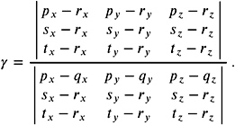
O3D( q, r, s, p ) determines the signed volume of the parallelepiped represented by four points p , q , r , and s ; the signed volume of the corresponding tetrahedron (see Figure 9.18) is given by
We have seen that the orientation test in 3D is somehow grounded in the orientation test of 2D. A geometric interpretation can be given as follows. Let us assume that we rotate the points p , q , r , and s to points p' , q' , r' , and s' so that p , q' , and r' lie in a plane parallel to the xy -plane and s' z has the largest z -coordinate. In other words, the vector (0 , , 1) is perpendicular to the plane spanned by p' , q' , and r' , and s' lies above the plane. Now O3D( p , q, r, s ) = O3D( p' , q' , r', s' ) is given by ˆ O2D( p' , q', r' ).
This holds in any dimension! For the orientation test in dimension d + 1, we rotate the points p 1 , p 2 , , p d +2 so that ![]() builds a plane perpendicular to the d + 1-dimensional vector (0 , , , 1) and p' d + 2 has the largest d + 1-coordinate. Now the sign of the orientation test of p 1 , p 2 , , p d + 2 in dimension d + 1 is given by the inverse sign of the orientation test of
builds a plane perpendicular to the d + 1-dimensional vector (0 , , , 1) and p' d + 2 has the largest d + 1-coordinate. Now the sign of the orientation test of p 1 , p 2 , , p d + 2 in dimension d + 1 is given by the inverse sign of the orientation test of ![]() in dimension d ; see also Generalization of the orientation and incircle tests to arbitrary dimensions later in this section. Thus, if p d + 2 sees the positive plane from above, the orientation test returns a negative value.
in dimension d ; see also Generalization of the orientation and incircle tests to arbitrary dimensions later in this section. Thus, if p d + 2 sees the positive plane from above, the orientation test returns a negative value.
Testing colinearity in 3D. O2D tests for colinearity in 2D, and O3D tests for coplanarity in 3D. So one might ask also whether three points in 3D are colinear. By ignoring the corresponding coordinates, we can project the points onto the xy -, yz - and xz -plane, respectively. We can choose any pair of the three planes and apply the O2D test for the corresponding points on both planes.
Let p = ( p x , p y , p z ), q = ( q x , q y , q z ), and r = ( r x , r y , r z ) denote three points in 3D. If all z -coordinates are the same, we can apply the O2D test for the points p = ( p x, p y ), q' = ( q x , q y ) , and r' = ( r x , r y ) . Otherwise, let p x z denote ( p x , p z ) in the xy -plane; p xz and p yz are defined analogously. We apply the orientation tests O2D( p xz , q xz , r xz ) and O2D( p yz , q yz , r yz ). The vertices are colinear in ![]() 3 iff both tests give zeros.
3 iff both tests give zeros.
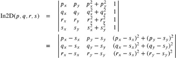
Incircle test in 2D. The incircle test in 2D points out whether a vertex s lies inside, outside, or on the circle passing through three vertices p , q , and r . Let Circle( p, q, r ) denote the set of points of the circle passing through the vertices p , q , and r . The expression In2D has the following semantic:

Fortunately, we are able to perform the incircle test by an orientation test in 3D. Let us assume that O2D( p, q, r ) is positive, and let us consider the following projection. A point a = ( a x , a y ) in the plane is projected onto the paraboloid P = {( x, y, x 2 + y 2 )( x, y ) ˆˆ ![]() 2 } by
2 } by
| (9.15) | |
We project all points of Circle( p, q, r ) onto the paraboloid P , which gives a set K on P ; see Figure 9.19. Now let us consider the orientations of the given planes. We assume that O2D( p, q, r ) is positive.
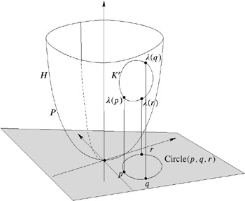
Figure 9.19: Projecting Circle(p, q, r) onto the paraboloid results in a set of points lying in a 2D plane.
The set Circle( p, q, r ) can be expressed by Circle( p, q, r ) = {( x, y )( x ˆ I x ) 2 + ( y ˆ I y ) 2 = l 2 }, where I x , I y , and l depend on p , q , and r ; see Circumcenter and circumradii of triangles in 2D and 3D later in this section. Therefore, we have
which shows that K is given by the intersection of P with a 2D plane in 3D, uniquely determined by ( q ), ( r ), and ( s ). Altogether, we have the following result.
Theorem 9.30. Let p, q, r, and s be points in ![]() 2 . Let E denote the 2D oriented plane passing through the points ( p ) , ( q ) , and ( r ) . Let O2D( p, q, r ) > . The point s lies
2 . Let E denote the 2D oriented plane passing through the points ( p ) , ( q ) , and ( r ) . Let O2D( p, q, r ) > . The point s lies
-
inside Circle( p, q, r ) if ( s ) lies below E (In2D( p, q, r, s ) > 0) ,
-
outside Circle( p, q, r ) if ( s ) lies above E (In2D( p, q, r, s ) > 0) , and
-
on Circle( p, q, r ) if ( s ) lies on E ( In2D( p, q, r, s ) = 0) .
Altogether, it suffices to evaluate the following determinant.
If O2D( p, q, r ) is negative, the sign of In2D( p, q, r, s ) is reversed , so that In2D( p, q, r, s ) is negative iff s is inside Circle( p, q, r ) and so on.
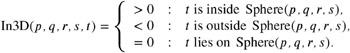
Insphere test in 3D. Similar to the incircle test, we are able to perform the insphere test in 3D by an orientation test in the fourth dimension. Let p , q , r , s , and t be five points in 3D. The incircle test should return whether t lies inside, outside, or on the sphere passing through the four points p , q , r , and s .
Let us assume that O3D( p, q, r, s ) is positive. Analogously, we project the points p , q , r , and s onto the 4D paraboloid ![]() and apply the orientation test in 3D to
and apply the orientation test in 3D to ![]() , and
, and ![]() .
.
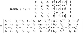
Let Sphere( p, q, r, s ) denote the sphere passing through p , q , r , and s . The semantic of In3D is as follows:
Generalization of the orientation and incircle tests to arbitrary dimensions. Let p 1 , p 2 , , p d + 1 be a sequence of d + 1 point in ![]() d , where
d , where ![]() . The orientation test in dimension d decides on which side of the oriented hyperplane passing through p 1 , p 2 , , p d the point p d + 1 lies. The value of the following determinant OdD is the signed volume of the simplex spanned by p 1 , p 2 , , p d + 1 , up to a constant depending on the dimension d .
. The orientation test in dimension d decides on which side of the oriented hyperplane passing through p 1 , p 2 , , p d the point p d + 1 lies. The value of the following determinant OdD is the signed volume of the simplex spanned by p 1 , p 2 , , p d + 1 , up to a constant depending on the dimension d .
| (9.16) | 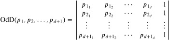 |
If the orientation test is performed more than once for the same hyperplane, it is worth storing some intermediate results. We can simply expand the determinant about the last row, thus obtaining a linear combination
where a i is determined by a determinant of the first d rows of Equation (9.16). More precisely, a 1 , a 2 , , a d + 1 represent the coefficients of the hyperplane passing through p 1 , p 2 , , p d ; i.e., the hyperplane passing through p 1 , p 2 , , p d is given by
Membership in a d -dimensional sphere can be calculated by an orientation test in dimension d + 1. If OdD( p 1 , p 2 , , p d + 1 ) is positive, we check whether p d + 2 is inside the sphere passing through p 1 , p 2 , , p d + 1 by evaluating the determinant
| (9.17) | 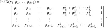 |
Similar to the preceding predicates for Equation (9.16) and Equation (9.17), there is an obvious rearrangement that makes use of simple transformations.
The correctness of the insphere test in dimension d can be proven with the same arguments as in Insphere test in 3D earlier in this section. It can be shown that the projections of d points ![]() onto the ( d + 1)-dimensional hyperparaboloid
onto the ( d + 1)-dimensional hyperparaboloid ![]() lie in a common d -dimensional hyperplane. A query point p d + 2 is inside the d -dimensional hypersphere passing through p 1 , , p d + 1 iff the corresponding projection of p d + 2 onto H lies below the hyperplane of
lie in a common d -dimensional hyperplane. A query point p d + 2 is inside the d -dimensional hypersphere passing through p 1 , , p d + 1 iff the corresponding projection of p d + 2 onto H lies below the hyperplane of
provided that p 1 , , p d +1 are oriented adequately.
Up to now, we have considered geometric predicates. Next, we turn to constructors. We will compute intersection results in various aspects. Although we can make use of robust transformations at the end of the calculations, we must transform the results back to the correct positions , which might cause cancellations (see also Section 9.4.1).
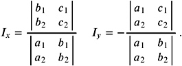
Intersection of lines in 2D and 3D. The intersection of two lines l 1 and l 2 depends on the representation of l 1 and l 2 . If l i = {( x, y ) ˆˆ ![]() 2 a i x + b i y + c i = 0}, then the intersection ( I x , I y ) is given by
2 a i x + b i y + c i = 0}, then the intersection ( I x , I y ) is given by
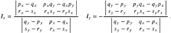
If l 1 is given by a pair of points ( p, q ) and l 2 is given by a pair of points ( r, s ), we can calculate a 1 = ( q y ˆ p y ), a 2 = ( s y ˆ r y ), b 1 = ( p x ˆ q x ), b 2 = ( r x ˆ s x ), c 1 = ( p y q x ˆ q y p x ), and c 2 = ( r y s x ˆ s y r x ), which gives
Equivalently, we can express the intersection point by the linear combination ( I x , I y ) = p + ( q ˆ p ), where
| (9.18) | 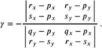 |
Note that the unique denominator
is zero iff l 1 and l 2 are parallel. Parallelism can be tested by evaluating a single determinant. The unique denominator is not equivalent to an orientation test in 2D but, for example, the numerator of Equation (9.18) is given by O2D( r, s, p ), which makes use of a transformation by p .
For ( I x , I y ) = p ˆ ( q ˆ p ), sometimes it might be helpful to rearrange p , q , r , and s . The denominator will change only its sign, but we may have less severe cancellations if ( I x , I y ) is close to p ; see also Section 9.4.1. Therefore, if ( I x , I y ) appears to be close to q , r , or s , we will swap the closest of the points to p .
For two lines in 3D, we can compute the intersection of the lines l 1 passing through p and q and l 2 passing through r and s by
Again, we can improve preciseness if ( I x , I y , I z ) is close to q , and eventually we swap p and q , which has no influence on the denominator.
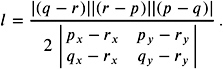
If there is no intersection, ( I x , I y , I z ) is a point on l 1 nearest to l 2 , and the distance between l 1 and l 2 is given by
Intersection of a line and a plane in 3D. Similar to the considerations in the previous section, we can express the intersection of a line passing through p and q and a plane passing through r , s , and t by ( I x , I y , I z ) = p ˆ ( q ˆ p ). where
As in the previous cases, it should be more robust to swap q and p if q is closer to ( I x , I y , I z ). We do not need to recompute the denominator in this case.
The denominator is zero iff the line and the plane run parallel. In this case, we have to check whether the line lies totally inside the plane by checking whether p is a linear combination of r , s , and t . This can be done by the Gaussian elimination technique of a system of linear equations; for a robust consideration of this technique, see for example [Schwarz 89].
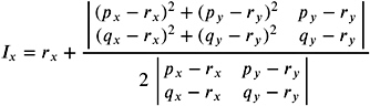
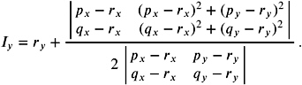
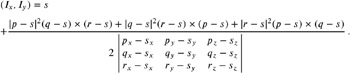
Circumcenter and circumradii of triangles in 2D and 3D. For example, the circumcenter of a circle passing through three points p , q , and r in the plane is relevant for the computation of a Voronoi diagram in 2D. If we consider the triangle spanned by p , q , and r , the circumcenter ( I x , I y ) is given by the intersection of the three perpendicular bisectors of the sides of the triangle where
and
The denominator represents O2D( p, q, r ), and the coordinates are unstable if the three points are almost colinear. The corresponding radius of the circle can be efficiently computed by
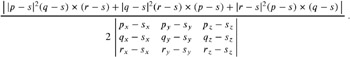
Altogether, we have Circle( q, r, s ) ={( x, y ) ˆˆ ![]() 2 ( x ˆ I x ) 2 + ( y ˆ I y ) 2 = l 2 }. The center of the triangle in 3D can be computed by
2 ( x ˆ I x ) 2 + ( y ˆ I y ) 2 = l 2 }. The center of the triangle in 3D can be computed by
Circumcenter and circumradii of a tetrahedron. The center ( I x , I y ) of the circumsphere of the tetrahedron expressed by four points p , q , r , and s in 3D is given by
The corresponding radius l reads
The denominator is equivalent to O3D( p, q, r, s ), and it is unstable if the four points are almost coplanar.
9.4.3. Efficient Evaluation of a Determinant
In the preceding section, we considered many predicates and constructors based on evaluation of determinants. The efficient evaluation of determinants is well supported by geometric libraries that support the exact geometric computation paradigm introduced in [Yap 93]; see also Section 9.3.4. For example, the LEDA library (http://www.algorithmic-solutions.com), the Core Library (http://www.cs.nyu.edu/exact/ core /), and the Real/Expr library (http://www.cs.nyu.edu/exact/realexpr/Det.html) support efficient determinant evaluations. On the other hand, robust and fast determinant calculations are also implemented in common computer algebra systems and can be supported by the use of exact number packages. See Section 9.7 for a detailed overview of existing packages. On the theoretical side, for an efficient and robust evaluation of the sign of determinants, see [Clarkson 92], [Kaltofen and Villard 04], or [Avnaim et al. 97].
EAN: N/A
Pages: 69