9.3. Geometric Computing and Arithmetic
| | ||
| | ||
| | ||
9.3. Geometric Computing and Arithmetic
Geometric algorithms are designed under the assumption of the Real Random Access Machine (Real RAM) computer model, which includes exact arithmetic on real numbers and allows a computer-independent analysis of complexity and running time in the famous O -notation.
For the Real RAM [Preparata and Shamos 90], we assume that each storage location is capable of holding a single real number and that the following operations are available at unit costs:
-
standard arithmetic operations (+, ˆ , —, /),
-
comparisons (<, ‰ , =, ‰ , ‰ , >),
-
extended arithmetic operations: k th root, trigonometric functions, exponential functions, and logarithm functions (if necessary).
Unfortunately , we cannot represent everyday decimal numbers in the binary system of computers. For example, the simple decimal number 0 . 1 has no exact representation in the binary system. We can give only a non-ending approximation by 0 . 0001100110011 , which is a short representation for 1 2 ˆ 4 + 1 2 ˆ 5 + 1 2 ˆ8 + 1 2 ˆ9 + 1 2 ˆ12 + 1 2 ˆ13 + . We conclude that exact arithmetic cannot be achieved for all decimal numbers directly.
Altogether, the Real RAM assumption does not always hold. Fast standard floating-point arithmetic running on modern microcomputers is accompanied with roundoff errors.
There are two main ways to overcome the problem: either we use fast standard floating-point arithmetic and try to live with the intrinsic errors or we have to implement the Real RAM by developing exact arithmetic. Sometimes, the solution is somewhere in between. As long as there are no severe problems, we can live with the roundoff errors of fast floating-point operations. If some serious problems arise, we will switch over to time-consuming exact operations.
The adaptive approach is also the basis for the paradigm called exact geometric computation (EGC); for example, considered in [Yap 97a] and [Burnikel et al. 99]. For EGC, the emphasis is on the geometric correctness of the output, rather than the exactness of the arithmetic. One tries to ensure that at least the decisions and the flow of the algorithm are correct and consistent. As long as no severe inconsistency appears, there is no need to perform cost-consuming exact calculations. EGC often is accompanied by an EGC library that guarantees exact comparisons; see Section 9.7 for a detailed discussion of existing packages.
First, in Section 9.3.1, we will have a look at the main properties of standard floating-point arithmetic available on almost every microcomputer. We will consider the cost impact of exact arithmetic in Section 9.3.2. Imprecise and adaptive arithmetic variants are presented in Section 9.3.3, and finally, the principles of EGC are shown in Section 9.3.4.
9.3.1. Floating-Point Arithmetic
Floating-point arithmetic for microcomputers is defined in the IEEE standards 754 and 854; see [Goldberg 91] and [IEEE 85].
For obvious reasons, hardware-supported arithmetic is restricted to binary operations. Therefore, the IEEE 754 standard is defined for the radix = 2. Fortunately, the standard includes rules for conversion to human decimal arithmetic. Therefore, with a little loss of precision, we can work with decimal arithmetic in the same manner. For example, programming languages make use of the conversion standard and give access to floating-point operations with radix = 10, which depend on hardware-supported fast floating-point operations with radix = 2.
The standard IEEE 854 allows either radix = 2 or radix = 10. In contrast to IEEE 754, it does not specify how numbers are encoded into bits. Additionally, the precisions single and double are not specified by particular values in IEEE 854. They have constraints for allowable values instead. With respect to encoding into bits and conversions to decimals, repeating the features of the standard IEEE 754 will give us some more insight.
The main advantage of standardization is that floating-point arithmetic is supported by almost every type of hardware in the same way. Thus, software implementations based on the standard are portable to almost every platform. With respect to the underlying arithmetic, floating-point operations should not produce different outputs on different platforms.
The floating-point arithmetic of a programming language should guarantee the same results on every platform and should be based on the standard. So, in some sense, a programming language analogously builds a standard of its own, following the rules of arithmetic and rounding as required in IEEE 754. Therefore, it is well justified to have a closer look at IEEE 754.
The main features of IEEE 754. We will give a short overview of the features and go into detail for some of them afterwards.
Definition 9.5. (Floating-point representation.) A floating-point representation consists of a base , a precision p , and an exponent range [ e min , e max ] = E . A floating-point number is represented by
where e ˆˆ E and 0 ‰ d i < . It represents the number
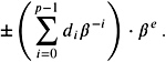
The representation is called normalized if d ‰ 0.
For example, the rational number 1/2 can be represented for p = 4 and = 10 by 0 . 500 or in a normalized form by 5 . 000 — 10 ˆ 1 .
A direct bit encoding for floating-point numbers is available only for = 2. Unfortunately, not all numbers can be represented exactly by floating-point numbers with = 2. For example, the rational 1/10 has the endless representation 1 . 100110011 — 2 ˆ4 .
For arbitrary , we have p possible significands and e max ˆ e min + 1 possible exponents. Taking one bit for the sign into account, we need
bits for the representation of an arbitrary floating-point number. The precise encoding is specified in IEEE 754 for = 2 and not specified for ‰ 2.
The IEEE 754 standard includes the following.
-
Representation of floating-point numbers: see Definition 9.5.
-
Precision formats: the precision formats are single, single extended, double, and double extended. For example, single precision makes use of 32 bits with p = 24, e max = +127, and e min = ˆ 126.
-
Format layout: the system layout of the precision formats is completely specified; see Section 9.3.1 for a detailed example of the single format.
-
Rounding: roundoff and roundoff errors for arbitrary floating-point arithmetic cannot be avoided, but the rounding rules should create reproducible results; see Section 9.3.1 for a detailed discussion of roundoff errors and rounding with respect to arithmetic operations.
-
Basic arithmetic operations: the standard includes rules for standard arithmetic. Addition, subtraction, multiplication, division, square root, and remainder have to be evaluated exactly first and rounded to nearest afterwards.
-
Conversions: conversions between floating-point and integer or decimal numbers have to be rounded and converted back exactly. For example, computation of 1/3 —3 should give the result 1 even though 1/3 must be rounded. Further discussions on conversion are given in Section 9.3.1.
-
Comparisons: comparisons between numbers with the predicates <, ‰ , or = have to be evaluated exactly also for different precisions.
-
Special values: some special numbers NaN, ˆ , and ˆ ˆ have an own fixed representation. Arithmetic with these numbers is standardized.
In the following, we will present the main ideas of the standard and its hardware realization.
Single format. The standard makes use of a format width of 32 bits for single precision p = 24 with e max = +127 and e min = ˆ 126. The first bit represents the sign, the next 8 bits represent the exponent, and the last 23 bits represent the significand. We will make use of the normalized form. Thus, 23 bits are sufficient to represent 24 significands if zero is a special value.
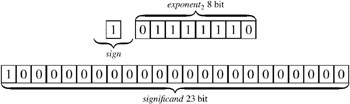
The exponent field should represent both negative and positive exponents. Therefore we use a bias, which is 127 here. An exponent of zero means that (0 ˆ bias) = ˆ 127 is the exponent, whereas an exponent of 255 results in the maximal exponent (255 ˆ bias) = 128. Altogether, the given example represents the number
Exponents of -127 (all exponents bits are zero) or +128 (all exponents bits are one) are reserved for special numbers; see the section on special values.
Roundoff errors. Roundoff errors can be expressed in an absolute and in a relative sense. In the following, a number z is referred to be exact if it is represented exactly with infinite precision with respect to the given radix . First, we specify how an exact value is represented as a floating-point value rounded by the round-to-nearest rule.
Definition 9.6. (Round to nearest.) An exact value z is rounded to the nearest floating-point number z if z is representable within the given precision p and z minimizes z ˆ z under all representable floating-point numbers.
If two representable floating-point numbers z and z exist with z ˆ z = z ˆ z , we make use of the so-called tie-breaking round-to-even rule, which takes the floating-point number with a biggest absolute value. Alternatively, we can apply a round-to-zero tie-breaking rule, which takes the floating-point number with the smallest absolute value.
For example, for p = 3 and basis = 10, the exact value z = 0 . 3158 is rounded to z = 0.316. The floating-point values 7.35 — 10 2 and 7 . 36 — 10 2 have the same absolute distance to z = 735 . 5. In this case, round-to-even will prefer 7 . 36 — 10 2 . The most natural way of measuring rounding errors is in units in last place (ulps).
Definition 9.7. (Units in last place.) The term units in the last place, ulp s for short, refers to the absolute error of a floating-point expression d .d 1 d 2 d p ˆ1 e with respect to the exact value z . That is, the absolute error is within
units in the last place.
For example, let precision p = 3 and basis = 10. If 3 . 12 — 10 ˆ 2 appears to be the result of a floating-point operation of the exact value z = 0 . 0314, we have an absolute error of 3 . 12 ˆ 3 . 1410 2 = 2 units in the last place. Similarly, if the exact value is z = 0 . 0312159, the absolute error is within 0 . 159 ulps. Let us consider an example with an exact value represented by infinite precision with the same basis. Let 3 . 34 — 10 ˆ 1 approximate the fractional expression 1/3, which, in turn , has an exact infinite representation 0 . 33333333 with = 10. The absolute error is given by = 0 . 666 ulps.
Note that rounding to the nearest possible floating-point value always has an error within ‰ 1/2 ulps. When analyzing the rounding error caused by various formulas, a relative error is a better measure. During the evaluation of arithmetic, subresults are successively converted by the round-to-nearest rule.
Definition 9.8. (Relative error.) The relative error of a given floating-point expression d .d 1 d 2 d p ˆ1 e with respect to the exact value z is represented by
For example, the relative error when approximating z = 0 . 0312159 by 3 . 12 — 10 ˆ 2 is 0 . 0000159 / . 0312159 ‰ˆ . 000005.
Let us consider the relative error of rounding to the nearest possible floating-point value. We can compute the relative error that corresponds to 1/2 ulp. When an exact number is approximated by the closest possible floating-point value d .d 1 d 2 d p ˆ1 e , the absolute error can be as large as
which is ![]() e . The numbers with values between e and e + 1 have the same absolute error of
e . The numbers with values between e and e + 1 have the same absolute error of ![]() e ; therefore, the relative error ranges between 1/2 ˆ p and
e ; therefore, the relative error ranges between 1/2 ˆ p and ![]() , which gives
, which gives
that is, the relative error corresponding to 1/2 ulps can vary by a factor of . Now ![]() =
= ![]() is the largest relative error possible when exact numbers are rounded to the nearest floating-point number,
is the largest relative error possible when exact numbers are rounded to the nearest floating-point number, ![]() is denoted also as the machine epsilon .
is denoted also as the machine epsilon .
Arithmetic operations. The standard includes rules for standard arithmetic operations such as addition, subtraction, multiplication, division, square root, and remainder. The main requirement is that the result of the imprecise arithmetic operation x op y of two floating-point values of precision p must be equal to the exact result of x op y , rounded to the nearest floating-point value within the given precision.
We will try to demonstrate how we can fulfill the requirement efficiently . For example, subtraction can be performed adequately with a fixed number of additional digits; similar results hold for other operations.
First, we will extract the problems. For example, for p = 3, = 10, x = 3 . 15 — 10 6 , and y = 1 . 25 — 10 ˆ 3 , we have to calculate
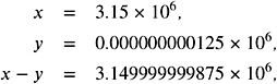
which is rounded to 3 . 15 — 10 6 . Obviously, we have used many unnecessary digits here. Efficient floating-point arithmetic hardware tries to avoid the use of many digits. Let us assume that, for simplicity, the machine shifts the smaller operand to the left and discards all extra digits. This will give
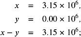
i.e., exactly the same result. Unfortunately, this does not work in the following example. For p = 4 and with x = 10 . 01 and y = 9 . 992, we achieve
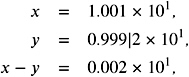
whereas the correct answer is 0.018. The computed answer differs by 200 ulps and is wrong in every digit. The next lemma shows how bad the relative error can be for the simple shift-and-discard rule.
Lemma 9.9. For floating-point numbers with precision p and basis computing subtraction using p digits, the relative error can be as large as ˆ 1 .
Proof: We can achieve a relative error of ˆ 1, if we choose x = 1 . 00 0 and ![]() with d = ( ˆ 1). The exact value is x ˆ y = ˆ p , whereas using p digits and shift-and-discard gives
with d = ( ˆ 1). The exact value is x ˆ y = ˆ p , whereas using p digits and shift-and-discard gives
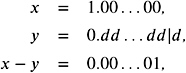
which equals ˆ p +1 . Thus, the absolute error is ˆ p ˆ ˆ p + 1 = ˆ p (1 ˆ ), and the relative error is ![]() .
.
Efficient hardware solution makes use of a restricted number of additional guard digits . As an example, we will show that just one extra digit achieves relatively precise results for subtraction. In general, three extra bits are sufficient for fulfilling the needs of the standard for all operations; see [Goldberg 91].
With one extra digit in the given example, we obtain
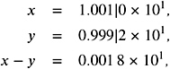
which gives the exact result 1 . 8 — 10 ˆ 2 . More generally , the following theorem holds for a single guard digit.
Theorem 9.10. For floating-point numbers with precision p and basis computing subtraction using p + 1 digits (one guard digit), the relative error is smaller than 2 ![]() , where
, where ![]() denotes the machine epsilon
denotes the machine epsilon ![]() .
.
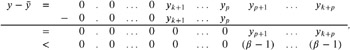
Proof: Let x > y . We scale x and y so that x = x .x 1 x 2 x p ˆ1 — and ![]() . Let y denote the part of y truncated to p + 1 digits. Thus, we have
. Let y denote the part of y truncated to p + 1 digits. Thus, we have
With an extra guard digit, x ˆ y is calculated by x ˆ y and rounded to be a floating-point number in the given precision. Thus, the result equals x ˆ y + where ‰ ![]() .
.
The relative error is given by
Additionally, we have
which gives
For k = 0 , ˆ 1, we are already finished, since x ˆ y is either exact or, due to the guard digit, rounded to the nearest floating-point value with a rounding error at most ![]() . So, in the following, let k > 0. If x ˆ y ‰ 1, we conclude
. So, in the following, let k > 0. If x ˆ y ‰ 1, we conclude
If x ˆ y < 1, we conclude = 0 because the result of x ˆ y has no more than p digits. The smallest value x ˆ y can achieve is
In this case, the relative error is bounded by
| (9.1) | 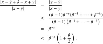 |
If x ˆ y ‰ 1 and x ˆ y < 1, we conclude x ˆ y = 1 and = 0. In this case, Equation (9.1) applies again. For = 2, the bound ![]() exactly achieves 2
exactly achieves 2 ![]() .
.
Note that a relative error of less than 2 ![]() already gives a good approximation but may be not precise enough for the standard, because 1/2 ulp < 2
already gives a good approximation but may be not precise enough for the standard, because 1/2 ulp < 2 ![]() .
.
In the following, we will denote the inexact versions of the operations of +, ˆ , —, and / by • , – , — , and ˜ . For convenience, we sometimes denote x — y by xy and x / y by ![]() , as usual.
, as usual.
The standard requires that for an arithmetic operation of two floating-point values in the given precision, the result will have a relative error smaller than the machine epsilon ![]() .
.
Therefore, for two floating-point values x and y , we have
| (9.2) | 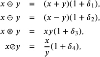 |
where i ‰ ![]() holds for i = 1, 2, 3, 4.
holds for i = 1, 2, 3, 4.
Conversions from and to decimal numbers. So far, you have seen that the decimal world and the binary world of the computer are not equivalent. Therefore, the standard provides for conversions from binary to decimal and back to binary, or from decimal to binary and back to decimal, respectively.
For example, the data type float of the Java programming language represents floating-point numbers with basis = 10 in a range from 3.4 — 10 38 with precision p = 6. This refers to the single format in IEEE 754. The maximal exponent in IEEE 754 is 128, and we have 2 128 = 3.40282 — 10 38 . The restriction of the precision to 6 refers to conversions from decimal to binary and back to decimal. It can be shown that if a decimal number x with precision 6 is transformed to the nearest binary floating-point x with precision 24, it is possible to transform x uniquely back to x . This cannot be guaranteed for decimal numbers with precision ‰ 7; see Theorem 9.12.
We exemplify the problems of a decimal-binary-decimal conversion cycle with rounding to nearest. Let us assume that binary and decimal are given by a similar finite precision. If decimal x is converted for the first time to the nearest binary x , we cannot guarantee that the nearest decimal of x results in the original value x ; see Figure 9.9.
Figure 9.9: Conversion cycle by rounding to nearest with a first-time error.
If the binary format has enough extra precision, rounding back to the nearest decimal floating-point value results in the original value; see Figure 9.10. In all cases, the error cannot increase; that is, repeated conversions after the first time give the same binary and decimal values.
Figure 9.10: Conversion cycle by rounding to nearest with the correct result.
We can calculate the corresponding sufficient precisions precisely and we will give a proof for the binary-decimal-binary conversion cycle.
Theorem 9.11. Let x be a binary floating-point number with precision 24. If x is converted to the nearest decimal floating-point number x w ith precision 8, we cannot convert x b ack to the original x by rounding to the nearest binary with precision 24. A precision of nine digits for the decimal is sufficient.
Proof: We consider the half- open interval [1000 , 1024) = [10 3 , 2 10 ). Binary numbers with precision 24 inside this interval obviously have 10 bits to the left and 14 bits to the right of the binary point. In the given interval, we have 24 different integer values from 1000 to 1023. Therefore, there are 24 — 2 14 = 393216 different binary numbers in the interval. Decimal numbers with precision 8 inside this interval obviously have four bits to the left and four bits to the right of the decimal point. Analogously, there are only 24 — 10 4 different decimal numbers in the same interval. So eight digits are not enough to represent each single-precision binary by a corresponding decimal.
To show that precision nine is sufficient, we will show that the spacing between binary numbers is always greater than the spacing between decimal numbers. Consider the interval [10 n , 10 n + 1 ]. In this interval, the spacing between two decimal numbers with precision 9 is 10 ( n +1)ˆ 9 . Let m be the smallest integer so that 10 n < 2 m . The spacing of all binary numbers with precision 24 in [10 n , 2 m ] is 2 ( m ˆ24) . The spacing gets larger from 2 m to 10 ( n +1) . Altogether, we have 10 ( n +1)ˆ9 < 2 ( m ˆ24 ) , and the spacing of the binary numbers is always larger.
For the decimal-binary-decimal conversion cycle, a similar result can be proven.
Theorem 9.12. Let x be a decimal floating-point number with precision 7. If x is converted to the nearest binary floating-point number x w ith precision 24, we cannot convert x b ack to the original x by rounding to the nearest binary value with precision 7. Precision 6 for the decimal value is sufficient.
Special values. IEEE 754 reserves exponent fields values of all 0s and all 1s to denote special values. We will exemplify the notions in the single format.
Zero cannot be represented directly because of the leading 1 in the normalized form. Therefore, zero is denoted with an exponent field of zero and a significand field of zero. Note that 0 and -0 are different values.
Infinity values + ˆ and ˆ ˆ are denoted with an exponent of all 1s and a significand of all 0s. The sign bit distinguishes between + ˆ and ˆ ˆ .
After an overflow, the system will be able to continue to evaluate expression by using arithmetic with + ˆ or ˆ ˆ .
NaN denotes illegal results, and they are represented by a bit pattern with an exponent of all 1s and a non-zero significand.
Arithmetic with special values allows operations to proceed after expressions run out of range. Arithmetic with a NaN subexpression always executes to NaN. Other operations can be found in the following table.
| Operation | Result |
|---|---|
| n / 0 | NaN |
| ˆ ˆ ˆ | NaN |
| ˆ / ˆ | NaN |
| ˆ — 0 | NaN |
| ˆ + ˆ | ˆ |
| ˆ — ˆ | ˆ |
| n / ˆ |
|
9.3.2. Exact Arithmetic
We have shown that fast floating-point arithmetic comes along with unavoidable roundoff errors. Therefore, sometimes using exact number packages is recommended. This so-called exact arithmetic approach refers to the fact that whenever a geometric algorithm starts, the corresponding objects have to be represented in a finite precision for the computer. In this sense, the input objects are always discrete. Therefore, one can guarantee the exact judgment of predicates by using a constant precision, though possibly much higher than the precision of the input.
A simple example is given in [Sugihara 00]. Let us assume that for the polyhedron problem of Section 9.1.2, we have points p i = ( x i , y i , z i ) ˆˆ I 3 with integer coordinates only. Now there is a fixed large positive integer K with
for all p i , and we are looking for the sign of
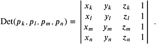
The Hadamard inequality [Gradshteyn and Ryzhik 00] states that the absolute value of the determinant of a matrix is bounded by the product of the length of the column vectors. More precisely, for every n — n A = ( a ij ) with a ij ˆˆ ![]() and A ‰ 0, we have
and A ‰ 0, we have ![]() . This means that
. This means that
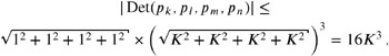
Hence, it suffices to use multiple-precision integers that are long enough to represent 16 K 3 .
As another example, we can consider the sweep algorithm for the arrangement in Section 9.1.1. The sweep is consistent as long as the comparison of the x -coordinates of intersections of line segments or endpoints of segments is correct. The x -coordinates of line segment intersections are given by values a/b where a and b denote 2 — 2 determinants with entries stemming from the subtraction of endpoint coordinates; see Section 9.4.2. More precisely, a is a multi-variate polynomial of degree 3 and b is a multi-variate polynomial of degree 2.
Therefore, we have to compute the sign of ![]() exactly, which is equivalent to the sign of a 1 b 2 ˆ a 2 b 1 . The last expression can be represented by a fifth degree multi-variate polynomial in the coordinates of the endpoints of line segments, see Section 9.4.2. Therefore, we have to adjust the precision of the arithmetic so that we can calculate five successive multiplications and some additions exactly. If the coordinates are given with precision k , it can be shown that it suffices to perform all computations with precision 6 k , due to the polynomial complexity of the sign test.
exactly, which is equivalent to the sign of a 1 b 2 ˆ a 2 b 1 . The last expression can be represented by a fifth degree multi-variate polynomial in the coordinates of the endpoints of line segments, see Section 9.4.2. Therefore, we have to adjust the precision of the arithmetic so that we can calculate five successive multiplications and some additions exactly. If the coordinates are given with precision k , it can be shown that it suffices to perform all computations with precision 6 k , due to the polynomial complexity of the sign test.
Unfortunately, multiple-precision computation may produce unnecessarily high computational costs. Additionally, the problem of degeneracy is not solved .
We summarize some useful exact number packages and analyze the performance impact.
Integer arithmetic. The idea of a multiple-precision integer system is very simple. An arbitrarily big, but finite, integer value can be stored exactly in the binary system of a computer if we allow enough space for its representation. Roughly speaking, we will use a software solution for the representation of numbers.
Big-integer, or more generally, big-number packages are part of almost every programming language (for example, Java, C++, Object Pascal, and Fortran) and are implemented for every computer algebra system (for example, Maple, Mathematica, and Scratchpad). Additionally, independent software packages are given (for example, BigNum, GMP, LiDIA, Real/exp, and PARI), and special computational geometry libraries (for example, LN, LEDA, LEA, CoreLibrary, and GeomLib) provide access to arbitrary precision numbers; more details are given in Section 9.7. The packages provide for number representation and standard arithmetic.
We consider the computational impact and the storage impact of big-integer arithmetic. They are closely related . If we need more bits for the representation of the inputs of an arithmetic operation, the operation costs increase.
Let us first consider the computational impact of big-integer arithmetic. Obviously, the evaluation of determinants is a central problem of computational geometry; see Section 9.1.2 and Section 9.4. A d — d determinant with integer entries can be naively computed by Gaussian elimination ; see [Schwarz 89]. We assume that every input value can be represented by at most b bits. Using floating-point arithmetic, we can eliminate the matrix entries with O ( d 3 ) b -bit hardware-supported operations. For exact integer arithmetic, we need to avoid divisions. Therefore, during the elimination process, the bit complexity of the entries may grow steadily by a factor of 2. The number of arbitrary precision operations is still bounded by O ( d 3 ), but the number of b -bit operations within these O ( d 3 ) operations can be exponential in d , because of increasing bit length. Altogether, the overhead of operations of the integer package can be very large. More precisely, we compare a running time of ![]() floating-point operations to an exponential running time of
floating-point operations to an exponential running time of ![]() big-integer operations.
big-integer operations.
On the other hand, for the number of additional bits needed for the evaluation of a multi-variate polynomial p of degree d . Keep in mind that we can represent a d — d determinant by such a polynomial. Let m be the number of monomials in p and let the coefficients of the monomial be bounded by a constant. The monomials of a multi-variate polynomial are the summands of the polynomial. For example, x 3 y 5 and x 4 y 2 and 7 are the monomials of p ( x, y ) = x 3 y 5 + x 4 y 2 + 7. It might happen that we need bd bits for the representation of a monomial, taking d multiplications of b bit values into account. Adding two monomials of complexity bd may increase the complexity by (at most) 1, adding four monomials of complexity bd may increase the complexity by (at most) 2, and so on. Altogether, the bit complexity may rise to bd + log m + O (1), whereas floating-point arithmetic is restricted to complexity b .
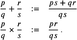
Rational arithmetic. A rational number can be represented by two integers. If we allow the arithmetic operations —, +, ˆ , and /, we can simply define rational arithmetic by integer arithmetic, using the well-known rules
Rational computing is unavoidable in the presence of integers. For example, the intersection of two lines each represented by integers may be rational; see Section 9.4.2. For obvious reasons, big-rational values normally are integrated into big-integer packages. Furthermore, big-number packages normally implement big-float values also; see, for example, BigNum, GNU MP, and LiDIA. As in the previous section, we should have a closer look at the computational cost and the bit complexity of rationals.
A rational p/q is represented by two integers. The bit complexity is given by the sum of the bit complexities of p and q . Unfortunately, a single addition may double the bit complexity. The addition of two b bit integer values results in a ( b + 1) bit integer, whereas the bit complexity of ![]() is the sum of the bit complexities of p/q and r/s . The bit complexity for evaluating a multi-variate polynomial of degree d with m monomials may rises to 2 m bd + O (1).
is the sum of the bit complexities of p/q and r/s . The bit complexity for evaluating a multi-variate polynomial of degree d with m monomials may rises to 2 m bd + O (1).
Let us consider the intersection example in Section 9.3.2. We have to compute the sign of an expression a 1 b 2 ˆ a 2 b 1 which is a multi-variate polynomial of degree 5, here with rational variables . If the corresponding integers are expressed by b bits, the number of sufficient bits rise to 2 5 b , which gives a factor of 10.
The computational cost impact of multi-precision rationals is similar to the cost of multi-precision integers. As already shown, in cascaded computations, the bit length of numbers may increase quickly. Therefore, the worst-case complexity of b bit operations can be exponential in size , whereas b bit floating-point operations will be bounded by a polynomial.
It was shown in [Yu 92] that exact rational arithmetic for modeling polyhedrals in 3D is intractable. The naive use of exact rational arithmetic for computing 2D Delaunay triangulations can be 10,000 times slower than a floating-point implementation; see [Karasick et al. 89].
Algebraic numbers. A powerful subclass of real and complex numbers is given by algebraic numbers. An algebraic number is defined to be the root of a polynomial with integer coefficients. The polynomial represents the corresponding number.
For example, the polynomial p ( x ) = x ˆ m shows that every integer m is algebraic. By p ( x ) = nx ˆ m , we can represent all rationals m/n . Additionally, we may have non-rationals. For example, ![]() is the root of p ( x ) = x 2 ˆ 2. Algebraic numbers can be complex; for example, i
is the root of p ( x ) = x 2 ˆ 2. Algebraic numbers can be complex; for example, i ![]() is a root of p ( x ) = x 2 + 2. Since and e are not algebraic, algebraic numbers define a proper subset of complex numbers.
is a root of p ( x ) = x 2 + 2. Since and e are not algebraic, algebraic numbers define a proper subset of complex numbers.
The sum, difference, product, and quotient of two algebraic numbers are algebraic, and the algebraic numbers therefore form a so-called field . In abstract algebra, a field is an algebraic structure in which the operations of addition, subtraction, multiplication, and division (except division by zero) may be performed, and the associative, commutative, and distributive rules that are familiar from the arithmetic of ordinary numbers hold.
For practical reasons, we are interested only in real numbers and mainly interested in the sign of an algebraic number.
Definition 9.13. (Algebraic number.) An algebraic number x ˆˆ ![]() is the root of an integer polynomial. It can be uniquely represented by the corresponding integer polynomial p ( x ) and an isolating interval [ a, b ] with a, b ˆˆ
is the root of an integer polynomial. It can be uniquely represented by the corresponding integer polynomial p ( x ) and an isolating interval [ a, b ] with a, b ˆˆ ![]() that identifies x uniquely.
that identifies x uniquely.
This means that the isolated interval representations ( x 2 ˆ 2 , [1 , 4]) and ( x 2 ˆ 2 , [0 , 6]) represent the same algebraic number. This is not a problem here. Let us briefly explain how arithmetic with algebraic numbers works.
Let and be algebraic, be a root of ![]() , and be a root of
, and be a root of ![]() . It is easy to show that the following holds:
. It is easy to show that the following holds:
-
ˆ is a root of
 ;
; -
1/ is root of
 ;
; -
+ is root of Res y ( p ( y ) , q ( x ˆ y ));
-
is root of
The resultant Res x ( p ( x ) , q ( x )) of two polynomials ![]() and
and ![]() in x is defined by the following determinant of an ( n + m ) — ( n + m ) matrix. We have m rows with entries a , a 1 , , a n and n rows with entries b , b 1 , , b m .
in x is defined by the following determinant of an ( n + m ) — ( n + m ) matrix. We have m rows with entries a , a 1 , , a n and n rows with entries b , b 1 , , b m .
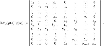
The corresponding matrix is denoted also as the Sylvester matrix. It is easy to show that, if Res x ( p ( x ) , q ( x )) = 0 holds, then p and q have a common root. Analogously, the resultant can be defined by
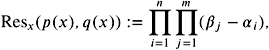
where i , for i = 1 , n are the roots of p ( x ) and i , for i = 1 , m are the roots of q ( x ); for more details, see [Davenport et al. 88].
With this definition, it is easy to see that
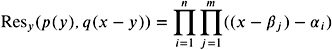
and
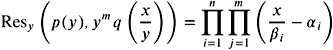
have roots i + j and i j , respectively. Altogether, algebraic numbers are closed under the operations +, ˆ , —, and /.
For a simple example, we choose p ( x ) = a + a 1 x and q ( x ) = b + b 1 x . Now, we have ![]() and
and ![]() , and
, and
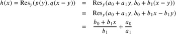
has root ![]() .
.
Algebraic numbers have the following interesting closure property.
Theorem 9.14. The root of a polynomial with algebraic coefficients is algebraic.
There are several ways of computing with algebraic numbers. With respect to geometric computing, we are mainly interested in the sign of real algebraic expressions and discuss two numerical approaches in Section 9.3.4. Several packages for algebraic computing are available; see Section 9.7 for a detailed discussion of existing packages.
9.3.3. Robust and Efficient Arithmetic
In this section, we will present some techniques for using fast arithmetic while trying to avoid serious errors. We will start with the popular but naive ![]() -tweaking method and then move on to more sophisticated techniques. The main idea is the use of adaptive executions; i.e., cost-consumptive computations are performed only in critical cases.
-tweaking method and then move on to more sophisticated techniques. The main idea is the use of adaptive executions; i.e., cost-consumptive computations are performed only in critical cases.
Epsilon comparison. Epsilon comparison is the standard model of almost every programmer. Every floating-point result whose absolute value is smaller than a (probably adjustable) threshold traditionally denoted by ![]() is considered to be zero. This works fine in many situations, but can never guarantee robustness. Epsilon comparison is not recommended in general. Epsilon comparison is known also as epsilon tweaking or epsilon heuristic . A value for epsilon is typically found by trial and error.
is considered to be zero. This works fine in many situations, but can never guarantee robustness. Epsilon comparison is not recommended in general. Epsilon comparison is known also as epsilon tweaking or epsilon heuristic . A value for epsilon is typically found by trial and error.
Formally, epsilon tweaking defines the following relation: a ~ b : a ˆ b < ![]() . Unfortunately, no
. Unfortunately, no ![]() can guarantee that ~ is an equivalence relation. From a ˆ b <
can guarantee that ~ is an equivalence relation. From a ˆ b < ![]() and b ˆ c <
and b ˆ c < ![]() , we cannot conclude that a ˆ c <
, we cannot conclude that a ˆ c < ![]() holds. So transitivity does not hold. Therefore, epsilon comparison can fail and can lead to inconsistencies and errors.
holds. So transitivity does not hold. Therefore, epsilon comparison can fail and can lead to inconsistencies and errors.
To make epsilon comparison a bit more robust, one should apply the following simple practical rules; see also [Michelucci 97, Michelucci 96] and [Santisteve 99].
-
It is useful to define several thresholds: one for lengths, another for areas, another for angle, and so on. Adjust them carefully to the problem situation.
-
Try to test special situations separately by simple comparisons. For example, for line segment intersection, we may check in advance, by comparison of the coordinates, that an intersection cannot occur.
-
Try to avoid unnecessary computations. For example, distances between points can be compared without the use of a erroneous square root operation.
-
Use exact data representation for comparisons. For example, an intersection may be represented by the numerical value and the corresponding segments. Two intersections should be compared with the original data.
-
Never use different representations of the same expression. This might introduce inconsistencies. Somehow, this contradicts the next item.
-
Rearrange predicates and expressions to avoid severe cancellation of digits. Use case distinctions for the best choice; this is the theme of Section 9.4.
Robust adaptive floating-point expressions. We want to make use of fast floating-point operations with fixed-precision p . We can assume that the input data has a fixed precision ‰ p . We follow the ideas and arguments in [Shewchuk 97]. Floating-point expressions with limited precision are expanded so that the error can be recalculated if necessary. In the following, we assume that and p are given.
Definition 9.15. (Expansion.) Let x i for i = 1 , n be floating-point numbers with respect to and p . Then
is called an expansion. x i are called components .
For example, let p = 6 and = 2. Then ˆ 11 + 1100 + ˆ 111000 is an expansion with three components. For our purpose, we consider so-called non-overlapping expansions.
Definition 9.16. (Non-overlapping floating-point numbers.) Two floating-point numbers x and y are non-overlapping iff the smallest significant bit of x is bigger than the biggest significant bit of y or vice versa.
For example, x = ˆ 110000 and y = 110 are non-overlapping. It is useful to consider non-overlapping expansions ![]() ordered by the absolute value of the subexpressions x i ; that is, x i > x i +1 for i = 1 , , ( n ˆ 1). In this case, the sign of x is determined by the sign of x 1 .
ordered by the absolute value of the subexpressions x i ; that is, x i > x i +1 for i = 1 , , ( n ˆ 1). In this case, the sign of x is determined by the sign of x 1 .
Definition 9.17. (Normalized expansion.) A normalized expansion ![]() has pairwise non-overlapping components x i and additionally x i > x i +1 for i = 1 , , ( n ˆ 1) holds.
has pairwise non-overlapping components x i and additionally x i > x i +1 for i = 1 , , ( n ˆ 1) holds.
As you will see, sometimes some of the inner components may become zero. In this case, we speak also of a normalized expansion iff the condition x i > x i +1 for i = 1 , , ( n ˆ 1) holds for all non-zero components.
The main idea is that we can expand floating-point arithmetic to floating-point arithmetic with expansions, thus being able to reconstruct rounding errors if necessary. In other words, instead of using more digits, we make use of more terms. In many cases, only a few terms are relevant. We try to present the main ideas of the expansion approach; more details can be found in [Shewchuk 97]. Arithmetic with expansions is based on the following observations.
According to the standard IEEE 754 for floating-point arithmetic (see Section 9.3.1, for example) for addition, the following holds:
where and err( a • b ) can be positive or negative. In any case, we have err( a • b ) ‰ 1/2 ulp( a • b ), since the standard guarantees exact arithmetic combined with the round-to-nearest rule and the round-to-even tie-breaking rule. Unfortunately, floating-point arithmetic breaks standard arithmetic rules such as associativity. For example, for p = 4 and = 2, we have ( 1000 • . 011 ) • . 011 = 1000 but 1000 • ( . 011 • . 011) = 1001.
We can make use of the ulp notation as a function of an incorrect result. It represents the magnitude of the smallest bit in the given precision. For example, for p = 4, we have ulp( ˆ 1001) = 1 and ulp(10) = 0 . 01. It seems to be natural to represent a + b by a non-overlapping expansion x + y with x = ( a • b ) and y = ˆ err( a • b ), provided that the error is representable within the given precision. We can construct non-overlapping expansions by addition using Algorithm 9.1.
| |
FastTwoSum( a, b ) ( a ‰ b )
x := a b b virtual := x a y := b b virtual return ( x, y )
| |
In the following, we assume = 2 and p is fixed. Some of the proofs will make use of = 2, which means that we cannot change the base. Fortunately, this is not a restriction. Either we make use of the conversion properties of the IEEE standard (see Section 9.3.1) or we must convert the input data of our problem by hand.
Theorem 9.18. Let a, b be floating-point numbers with a ‰ b . The algorithm FastTwoSum computes a non-overlapping expansion x + y = a + b, where x represents the approximation a • b and y represents the roundoff error ˆ err( a • b ).
Before we prove Theorem 9.18, we consider the following example for p = 4 and = 2 with a = 111100 and b = 1001 . We have
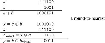
which results in a non-overlapping representation 1001000 + ˆ 11 = 1000101 = a + b . Note that FastTwoSum uses a constant number of p -bit floating-point operations.
First, we prove some helpful lemmata.
Lemma 9.19. Let a and b be floating-point numbers.
-
If a ˆ b ‰ b and a ˆ b ‰ a , then a – b = a ˆ b.
-
If b ˆˆ [ a/ 2 , 2 a ] , then a – b = a ˆ b.
Proof: For the first part, we assume without loss of generality that a ‰ b . The leading bit of a ˆ b is no bigger in magnitude than the leading bit of b ; the smallest bit of a ˆ b is no smaller than the smallest bit of b . Altogether, a ˆ b can be expressed with p bits. For the second part, without loss of generality, we assume a ‰ b . The other case is symmetric using ˆ b – ˆ a . We conclude that b ˆˆ [ ![]() , a ]. And we have sign( a ) = sign( b ). Therefore, we have a ˆ b ‰ b ‰ a and we apply the first part of the lemma.
, a ]. And we have sign( a ) = sign( b ). Therefore, we have a ˆ b ‰ b ‰ a and we apply the first part of the lemma.
Now we can prove that the following subtraction is exact.
Lemma 9.20. Let a ‰ b and x = a + b +err( a • b ) then b virtual := x – a = x ˆ a .
Proof: Case 1. If sign( a ) = sign( b ) or if b < ![]() holds, we conclude that x ˆˆ [
holds, we conclude that x ˆˆ [ ![]() , 2 a ], and we apply Lemma 9.19 to ˆ ( a – x ).
, 2 a ], and we apply Lemma 9.19 to ˆ ( a – x ).
Case 2. If sign( a ) ‰ sign( b ) and b ‰ ![]() , we have b ˆˆ [ ˆ
, we have b ˆˆ [ ˆ ![]() , ˆ a ]. Now x is computed exactly because x = a • b = a – ˆ b equals a ˆ ˆ b = a + b by Lemma 9.19. Thus, b virtual := x – a = ( a + b ) – a = b.
, ˆ a ]. Now x is computed exactly because x = a • b = a – ˆ b equals a ˆ ˆ b = a + b by Lemma 9.19. Thus, b virtual := x – a = ( a + b ) – a = b.
Lemma 9.21. The roundoff error err( a • b ) of a + b can be expressed with p bits.
Proof: Without loss of generality, we assume a ‰ b , and we have a • b is the floating-point number with p bits closest to a + b . But a is a p -bit floating-point number. The distance between a • b and a + b cannot be greater then b , altogether err( a • b ) ‰ b ‰ a , and the error is representable with p bits.
Now we can prove Theorem 9.18.
Proof: The first assignment gives x = a + b + err( a • b ). For the second assignment, we conclude b virtual = x – a = x ˆ a from Lemma 9.20. The third assignment is computed exactly also, because b – bv irtual = b + a ˆ x = ˆ err( a • b ) can be represented by p bits; see Lemma 9.21. In either case, we have y = ˆ err( a • b ) and x = a + b + err( a • b ). Exact rounding guarantees that y ‰ 1/2 ulp( x ); therefore, x and y are non-overlapping.
The algorithm FastTwoSum stems from Dekker [Dekker 71]. A more convenient algorithm, TwoSum by Knuth [Knuth 81], does not require a ‰ b and avoids cost-consuming comparisons.
Without a proof, TwoSum analogously computes a normalized expansion x + y , where y represents the error term. Additionally, there are analogous results for constructing expansions for subtraction and products of two floating-point numbers. We do not go into detail and refer to [Shewchuk 97].
Up to now, we have constructed a single expansion by addition. Obviously. we have to provide for arithmetic between expansions. That is, for two normalized expansions e and f with m and n components, respectively, we want to compute a normalized expansion h with e + f = h . First, we show that we can extend a normalized expansion by addition of a single p -bit number. The computation scheme is shown in Figure 9.11. It might happen that some components become zero, but non-zero components are still ordered by magnitude. If FastTwoSum should be applied, we have to make a case distinction in Algorithm 9.3.
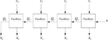
Figure 9.11: The scheme of the procedure GrowExpansion. (Redrawn and adapted courtesy of Jonathan Richard Shewchuk [Shewchuk 97].)
Theorem 9.22. Let ![]() be a normalized expansion with m components and let b be a p ‰ 3 bit floating-point number. The algorithm GrowExpansion computes a normalized (up to zero components) expansion
be a normalized expansion with m components and let b be a p ‰ 3 bit floating-point number. The algorithm GrowExpansion computes a normalized (up to zero components) expansion
with O ( m ) p-bit floating-point operations.
| |
TwoSum( a, b )
x := a b b virtual := x a a virtual := x b virtual b roundoff := b b virtual a roundoff := a a virtual y := a roundoff b roundof f return ( x, y )
| |
| |
GrowExpansion ![]()
Q := b for i := 1 TO m do TwoSum( Q i 1 , e i ) end for h m + 1 := Q m return h = ( h 1 , h 2 , , h m +1 ) | |
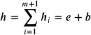
Proof: First, we show by induction that the invariant
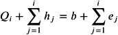
holds after the i th iteration of the for statement. Obviously, the invariant holds for i = 0 with Q = b . Now assume that ![]() holds, and we compute Q i ˆ 1 + e i = Q i + b i in line 3. Thus, we have
holds, and we compute Q i ˆ 1 + e i = Q i + b i in line 3. Thus, we have ![]() , and the induction step is shown.
, and the induction step is shown.
At the end, we obtain ![]() .
.
It remains to show that the result is normalized; that is, ordered by magnitude and non-overlapping. For all i , the output of TwoSum has the property that h i and Q i do not overlap. From the proof of Lemma 9.21, we know that h i = err( Q i ˆ1 • e i ) ‰ e i . Additionally, e is a non-overlapping expansion whose non-zero components are arranged in increasing order. Therefore, h i cannot overlap e i + 1 , e i + 2 , . The next component of h is constructed by summing Q i with component e i +1 , the corresponding error term h i + 1 is either zero or must be bigger and non-overlapping with respect to h i . Altogether, h is non-overlapping and increasing (except for zero components of h).
Let us consider a simple example for p = 5. Let e = e 1 + e 2 = 111100 + 1000000 and b = 1001. We have TwoSum( Q , e 1 ) = TwoSum( 1001 , 111100 ) = (1000100 , 1) = ( Q 1 , h 1 ) and TwoSum( Q 1 , e 2 ) = TwoSum( 1000100 , 1000000 ) = (10001000 , ˆ 100) = ( Q 2 , h 2 ) and h 3 = 1000100. Thus, calling GrowExpansion( e, b ) results in 10001000 + ˆ 100 + 1 .
Finally, we are able to add two expansions by following the ExpansionSum procedure. The scheme of ExpansionSum is shown in Figure 9.12.
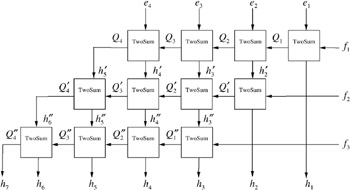
Figure 9.12: The addition scheme of ExpansionSum for two expansions
Theorem 9.23. Let ![]() be a normalized expansion with m components and
be a normalized expansion with m components and ![]() be a normalized expansion with n components. Let b be a p ‰ 3 bit floating-point number. The algorithm GrowExpansion computes a normalized expansion
be a normalized expansion with n components. Let b be a p ‰ 3 bit floating-point number. The algorithm GrowExpansion computes a normalized expansion
with O ( mn ) p-bit floating-point operations.
| |
ExpansionSum ![]()
h := e for i := 1 TO n do ( h i , h i +1 , , h i + m ) := GrowExpansion(( h i , h i +1 , ..., h i + m 1 ) , f i ) end for return h = ( h 1 , , h m + n )
| |
Proof: We give a proof sketch here. It can be shown by simple induction that ![]() . Following the addition scheme of Figure 9.12 one can prove successively that
. Following the addition scheme of Figure 9.12 one can prove successively that ![]() are non-overlapping and increasing for j = 1 , ( n ˆ 1).
are non-overlapping and increasing for j = 1 , ( n ˆ 1).
| |
TwoProduct( a, b ) ( a and b are p -bit floating-point values)
x := a b ( a x , a y ) := Split( b x ,b y ) := Split
err 1 := x ( a x b x ) err 2 := err 1 ( a y b x ) err 3 := err 2 ( a x b y ) y := ( a y b y ) err 3 return ( x, y )
| |
Analogous results can be proven for subtraction since we did not take the sign of the expressions into account. Therefore, there exists an algorithm TwoDiff that computes a non-overlapping expansion x + y = a – b ˆ err( a – b ) = a ˆ b . Furthermore, there is an algorithm ExpansionDiff that computes a normalized expansion ![]() for two normalized expansions
for two normalized expansions ![]() and
and ![]() .
.
For more sophisticated expressions, simple multiplications and scalar multiplication should be available. It was shown in [Shewchuk 97] that corresponding algorithms TwoProduct and ScaleExpansion exist. Technically, TwoProduct makes use of a splitting operation Split; see Algorithm 9.6. Here, a floating-point value is split into two half-precision values, and afterwards four multiplications of the corresponding fragments are performed; see [Dekker 71] and [Shewchuk 97]. In turn, ScaleExpansion makes use of TwoSum and TwoProduct.
Theorem 9.24. Let a and b be two floating-point values with p ‰ 6 . There is an algorithm TwoProduct that computes a non-overlapping expansion x + y = a — b ˆ err( a — b ) = a ˆ b with x = a — b and y = ˆ err( a — b ) .
| |
Split( a, s ) ( a represents a p -bit floating-point value, and s is a splitting value with p/ 2 ‰ s ‰ p ˆ 1)
c := (2 s + 1) a big := c a x := c big y := a x return ( x, y )
| |
| |
ScaleExpansion ![]()
( Q 2 , h 1 ) := TwoProduct( e 1 , b ) for i := 2 TO m do ( S i , s i ) := TwoProduct( e i , b ) ( Q 2 i 1 , h 2 i 2 ) := TwoSum( Q 2 i 2 , s i ) ( Q 2 i , h 2 i 1 ) := FastTwoSum( S i , Q 2 i 2 ) end for h 2 m := Q 2 m return ( h 1 , h 2 , , h 2 m ) | |
Theorem 9.25. Let ![]() be a normalized expansion with p ‰ 6 and let b be a floating-point value. There is an algorithm ScaleExpansion that computes a normalized expansion
be a normalized expansion with p ‰ 6 and let b be a floating-point value. There is an algorithm ScaleExpansion that computes a normalized expansion ![]() with O ( m ) p-bit floating-point operations.
with O ( m ) p-bit floating-point operations.
We omit the proofs and refer to [Shewchuk 97] or [Shewchuk 96], where some other useful operations are presented. For example, we have seen that some of the components may become zero. So, it is highly recommended that we compress a given expansion.
Theorem 9.26. Let ![]() be a normalized expansion with p ‰ 3 . Some of the components may be zero. There is an algorithm Compress that computes a normalized expansion
be a normalized expansion with p ‰ 3 . Some of the components may be zero. There is an algorithm Compress that computes a normalized expansion ![]() with non-zero components if e ‰ . The largest component h n approximates e with an error smaller than ulp( h n ) .
with non-zero components if e ‰ . The largest component h n approximates e with an error smaller than ulp( h n ) .
Compress guarantees that the largest component is a good approximation for the value of the whole expression.
Now we will try to demonstrate how expansion arithmetic is used for adaptive evaluations of geometric expressions. We consider the following simple example stemming from [Shewchuk 97] and explain the main construction rules. For convenience, we make use of an expression tree. An expression tree is a binary tree that represents an arithmetic expressions. The leaves of the tree represent constants, whereas every inner node represents a geometric operation of its children. In the case of expansion arithmetic, the leaves consist of p -bit floating-point values.
Let us assume that we want to compute the square of the distance between two points a = ( a x , a y ) and b = ( b x , b y ). That is, we need to compute ( a x ˆ b x ) 2 + ( a y ˆ b y ) 2 . In a first step, we construct expansions x 1 + y 1 = ( a x ˆ b x ) and x 2 + y 2 = ( a y ˆ b y ) by a construction algorithm TwoSum. We conclude from Theorem 9.18 that
| |
Compress ![]()
Q := e m Bottom := m for i := m 1 Down TO 1 d ( Q, q ) := FastTwoSum( Q, e i ) if q then g Bottom := Q Bottom := Bottom 1 Q := q end if end for g Bottom := Q Top := 1 for i := Bottom +1 TO m d ( Q, q ) := FastTwoSum( g i , Q ) if q then h Top := Q Top := Top 1 end if end for h Top := Q n := Top return ( h 1 , h 2 , , h n )
| |
-
y 1 = err( a x – b x ) ‰
 x 1 ,
x 1 , -
y 2 = err( a y – b y ) ‰
x 2 , -
x 1 = a x – b x ,
-
x 2 = a y – b y ,
where ![]() represents the machine epsilon. Now ( a x ˆ b x ) 2 + ( a y ˆ b y ) 2 equals
represents the machine epsilon. Now ( a x ˆ b x ) 2 + ( a y ˆ b y ) 2 equals ![]() , and we have the following magnitudes :
, and we have the following magnitudes :
-
 ,
, -
2( x 1 y 1 + x 2 y 2 ) ˆˆ O (
), and -
 .
.
More generally, let T i be the sum of all products that contain i y variables. Then T i has magnitude O ( ![]() i ). Now we can build different expression trees that collect T i terms in an appropriate way. A simple incremental adaptive approach is shown in Figure 9.13. The approximation A i contains all terms with size O (
i ). Now we can build different expression trees that collect T i terms in an appropriate way. A simple incremental adaptive approach is shown in Figure 9.13. The approximation A i contains all terms with size O ( ![]() i ˆ 1 ) or larger. A 3 is the correct result. More precisely, the approximation A i is computed by the sum of the approximation A i ˆ 1 and T i . In the following, we will refer to this as the simple incremental adaptive method. It collects the error terms with respect to the lowest level of the expression tree, i.e., with respect to the input values. Note that we have already sorted the input terms by error magnitude.
i ˆ 1 ) or larger. A 3 is the correct result. More precisely, the approximation A i is computed by the sum of the approximation A i ˆ 1 and T i . In the following, we will refer to this as the simple incremental adaptive method. It collects the error terms with respect to the lowest level of the expression tree, i.e., with respect to the input values. Note that we have already sorted the input terms by error magnitude.
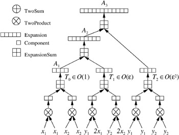
Figure 9.13: The simple incremental adaptive approach collects the errors by magnitude on the lowest level. (Redrawn and adapted courtesy of Jonathan Richard Shewchuk [Shewchuk 97].)
We can repeat this principle in higher levels. For example, the result of TwoProduct( x 1 , x 1 ) = x + y consists of an error term y with magnitude O ( ![]() ). The error terms T i can be computed adaptively. In Figure 9.14, we take incremental adaptivity to an extreme, recollecting the O (
). The error terms T i can be computed adaptively. In Figure 9.14, we take incremental adaptivity to an extreme, recollecting the O ( ![]() i ) error terms in all levels. This method can be denoted as the full incremental adaptive method. For an approximation A i with error O (
i ) error terms in all levels. This method can be denoted as the full incremental adaptive method. For an approximation A i with error O ( ![]() i ), we need to approximate the error terms with error O (
i ), we need to approximate the error terms with error O ( ![]() i ). Since the error term T k itself has magnitude O (
i ). Since the error term T k itself has magnitude O ( ![]() k ) , we have to approximate T k up to an error of O (
k ) , we have to approximate T k up to an error of O ( ![]() i ˆ k ). In this sense, this approach is economical, especially if the needed accuracy is known in advance.
i ˆ k ). In this sense, this approach is economical, especially if the needed accuracy is known in advance.
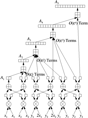
Figure 9.14: The full incremental adaptive approach collects the errors by magnitude on every level. (Redrawn and adapted courtesy of Jonathan Richard Shewchuk [Shewchuk 97].)
On the negative side, the full incremental adaptive approach leads to expression trees with a high complexity, since we keep track of many small error terms. Therefore, sometimes a better adaptive method with intermediate complexity could be more convenient. The intermediate incremental adaptive approach makes use of the approximation A i of the simple incremental method. Additionally, for the approximation of A i + 1 , we compute a simple approximation ct( T i ) of T i , thus obtaining an intermediate approximation C i = A i + ct( T i ). The method is illustrated in Figure 9.15. Sometimes, the correction term is already good enough, and the next error term is not computed.
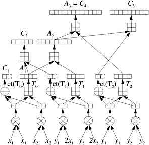
Figure 9.15: The intermediate incremental adaptive approach approximates the errors T i in a correction term. (Redrawn and adapted courtesy of Jonathan Richard Shewchuk [Shewchuk 97].)
Note that we can use the three construction schemes for the computations of the geometric predicates and expressions presented in Section 9.4. An extended example for the orientation test is given in [Shewchuk 97].
Floating-point filters. The previous adaptive approach makes use of floating-point arithmetic only, whereas the next two approaches come along with an exact arithmetic package. The exact package is used if a sufficient precision cannot be guaranteed by floating-point arithmetic.
We would like to reduce the number of exact calculations. In the floating-point filter approach, we replace the exact evaluation of an expression by the evaluation of guaranteed upper and lower bounds on its value. When the sign of the expression is needed and the bounding interval does not contain zero, then the sign is known. Otherwise, we have to use higher precision or exact arithmetic.
We follow the lines of [Mehlhorn and Nher 94]. Let us assume that we need to evaluate the sign of an arithmetic expression E . First, we will compute an approximation E using fixed-precision floating-point arithmetic. Additionally, we analyze the absolute error to obtain an error bound with E ˆ E ‰ . Obviously, if = 0 or E > , the signs of E and E are the same. Otherwise, if ‰ 0 and E ‰ , the filter approach failed, and we have to recompute E more precisely.
Let the cost for computing E be denoted by Exact. Let the cost of computing E and be denoted by Filter. Finally, let probFilter denote the probability that the filter fails. In this case, the expected cost is Filter + probFilter — Exact. Minimizing Filter and minimizing probFilter are two contradicting goals. In an extreme case, we will have Filter = 0 and probFilter = 1 if there is no filter, and on the other side, Filter = Exact and probFilter = 0 if the exact value represents the filter.
Let us consider some examples for an inductive construction of appropriate error bounds. We assume that the error bounds a and b and the approximations a and b for a and b have already been computed. The approximations result from floating-point operations. If we need to compute an error bound for c = a + b , we can make use of the following technique.
We compute c := a • b , and we have
| (9.3) | 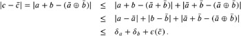 |
This means that the error bound c can be given by the sum of the error bounds plus ![]() c , where
c , where ![]() denotes the machine error, as usual. If the sign of the expression is needed, we compare the absolute value of the approximation c with the error estimate.
denotes the machine error, as usual. If the sign of the expression is needed, we compare the absolute value of the approximation c with the error estimate.
Similarly, we can design a floating-point filter for multiplications. For concreteness, we assume that c = a — b have to be computed under the same prerequisites. Thus, we conclude that for c := a — b , the error is bounded as follows :
| (9.4) | 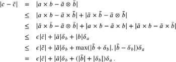 |
Altogether, c is computed by three multiplications and some additions.
The presented method is called dynamic error analysis because we dynamically take some additional operations (for example, computing b ˆ b ) into account. Actually, we have to perform floating-point operations for c , so the situation is a bit more complicated.
Other filter methods try to use error bounds that can be almost precomputed for the complete expression structure. In this case, only the floating-point operations of the expression have to be computed. Such methods are called static error analysis or semi-dynamic error analysis , and they require a few additional operations. Static and semi-dynamic filters make use of a priori estimates of the magnitude of the corresponding results.
For example, as shown previously, the error c ˆ c for c := a • b is given by a ˆ a + b ˆ b + a + b ˆ ( a • b ). Let us assume that there are already inductive bounds ind a ,ind b , max a , and max b , so that b ˆ b ‰ ind b max b and a ˆ a ‰ ind a max a . Here, max b is a binary estimate of the magnitude of b , and ind b refers to the depth of the inductive estimation. As a consequence, the error estimate for c ˆ c can be given by ind c max c with max c := max a + max b and ![]() . We can represent any geometric expression E by its expression tree; see Figure 9.16 or Section 9.3.3. Let us assume that we have floating-point arithmetic with = 2 and precision p . For every leaf x of the expression tree E , we initialize the inductive process by ind x = 2 ˆ( p + 1) = 1/2
. We can represent any geometric expression E by its expression tree; see Figure 9.16 or Section 9.3.3. Let us assume that we have floating-point arithmetic with = 2 and precision p . For every leaf x of the expression tree E , we initialize the inductive process by ind x = 2 ˆ( p + 1) = 1/2 ![]() and an appropriate value for max x . In the static version, we may choose the maximal power of two, bounding all input values x . In the semi-dynamic version, we may choose to take the magnitude of every leaf x into account; thus, we may set
and an appropriate value for max x . In the static version, we may choose the maximal power of two, bounding all input values x . In the semi-dynamic version, we may choose to take the magnitude of every leaf x into account; thus, we may set ![]() . In both cases, the error estimate for E is completely determined. Similar results hold for multiplications and other simple operations.
. In both cases, the error estimate for E is completely determined. Similar results hold for multiplications and other simple operations.
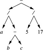
Figure 9.16: The expression tree of
Static error analysis is used in the LN package of [Fortune and Van Wyk 93], whereas semi-dynamic error analysis is part of LEDAs floating-point operations; see [Mehlhorn and Nher 00]. Floating-point filters can be easily computed in advance; unfortunately, it might happen that the estimate is two pessimistic.
Lazy evaluation. Lazy evaluation makes use of a well-suited representation of arithmetic expression. The arithmetic expression is represented twice: once by its formal definition, i.e., its expression tree, and once by an approximation that is an arbitrary precision floating-point number together with an error bound. As long as the approximation is good enough, we use it. If we can no longer guarantee the sign of an expression by its approximation, we will increase the precision and use the expression tree for a better approximation.
Lazy evaluation is normally defined for integer arithmetic and rational arithmetic, and comes along with an arbitrary precision integer or rational arithmetic package. Approximations are computed by floating-point arithmetic. The floating-point approximation and its error bound can be expressed also by a floating-point interval that represents the approximation.
Let us assume that we use a package of arbitrary precision rationals. As already explained, a lazy number for the arithmetic expression ![]() is given by the expression tree of E (see Figure 9.16) and an approximation interval, say [ ˆ 9 . 23 — 10 ˆ 3 , 2 . 94 — 10 2 ]. Here, a , b , and c represent expression trees of lazy numbers.
is given by the expression tree of E (see Figure 9.16) and an approximation interval, say [ ˆ 9 . 23 — 10 ˆ 3 , 2 . 94 — 10 2 ]. Here, a , b , and c represent expression trees of lazy numbers.
Inductively, the expression tree is either an integer (or a constant) or an operator together with pointers to its arguments, i.e., references to other expression trees. Note that sometimes the expression tree may become a directed acyclic graph (DAG). For example, in Figure 9.16, assume that b ‰ a .
Elementary operations for lazy numbers are performed by the following steps.
-
Allocate a new tree (DAG) node for the result of the operation.
-
Compute the floating-point interval with the interval arithmetic operations, see below.
-
Register the name of the operation, the pointers to the operands, and the given interval at the given node.
In these steps, no exact computations will be performed. Let us assume that we have lazy numbers a and b . In the following cases, we will have to evaluate the intervals or expressions more precisely.
-
The sign of a is needed and the floating-point interval contains 0.
-
We have to compare a and b but the intervals do overlap.
-
The lazy number a belongs to number b , and b has to be determined more precisely.
It might happen that a lazy number is never evaluated exactly. We still have to create the approximation intervals for lazy numbers. We assume that all lazy numbers are bounded in magnitude by the maximal and minimal representable floating-point values M and ![]() on the machine. More precisely, we require x ˆˆ ] ˆ M, ˆ
on the machine. More precisely, we require x ˆˆ ] ˆ M, ˆ ![]() [ ˆ {0} ˆ ] +
[ ˆ {0} ˆ ] + ![]() , + M [ for every lazy number x .
, + M [ for every lazy number x .
For a floating-point number x , let ˆ ( x ) denote the next smallest representable floating-point number on the machine. Representable means representable within the given precision p , and the next smallest means smaller with respect to x . ˆ ( x ) denotes the next biggest representable floating-point number on the machine. For example, for p = 4 and x = 1, we have ˆ ( x ) = 0.9999 and ˆ ( x ) =1.001.
It is easy to show that for all operators + , — , ˆ , and / and their corresponding floating-point versions ![]() ,
, ![]() ,
, ![]() , and
, and ![]() , the following inequalities hold:
, the following inequalities hold:
and
Therefore, we conclude that for the construction of lazy numbers, we make use of the intervals [ ˆ ( a ![]() b ), ( a
b ), ( a ![]() b )] computed by floating-point arithmetic.
b )] computed by floating-point arithmetic.
Arithmetic with floating-point intervals for lazy numbers can be done as follows. Let x and y be lazy numbers with intervals I x = [ a x , b x ] and I y = [ a y , b y ].
-
I x + y = [ ˆ ( a x
 a y ), ( b x b y )]
 -
I x — y = [ ˆ ( m ) , ( M )] where m ( M ) is the minimum (maximum) of { a x
 a y , a x b y , b x a y , b x b y }
 -
I ˆ x = [ ˆ b x , ˆ a x ]
-

It is easy to see that the intervals may grow successively after some operations. Only precise evaluation can stop this process.
The natural way for the (interval) evaluation of a lazy expression starts at the leaves of the trees and successively propagates the results or intervals to the top (root) of the tree. During the evaluation process, some of the exact evaluated expressions may become useless. Therefore, a lazy arithmetic package should make use of a garbage collector. The lazy arithmetic package LEA [Benouamer et al. 93] is implemented in C++ and consists of three modules: an interval arithmetic module, a DAG module, and an exact rational arithmetic package.
Finally, we discuss the main advantage of lazy arithmetic versus pure floating-point filters. Let us assume that the needed precision varies a lot, i.e., sometimes low precision is enough, and in the worst case, high precision is needed. Lazy arithmetic is well suited for this situation. We can increase the precision of the calculations successively until finally the sign of the expression is determined by an interval. Floating-point filters do not support this adaptive approach.
Separation bounds for algebraic expressions. Another well suited adaptive arithmetic approach separates an arithmetic expression from zero. Similar to the previous sections we would like to evaluate the sign of an algebraic geometric expression given in an expression DAG. We discuss simple separation bound sfor algebraic numbers expressed by the operations +, ˆ , —, /, and ![]() for arbitrary integer k .
for arbitrary integer k .
Definition 9.27. (Separation bound.) Let E be an arithmetic expression with operators +, ˆ , —, /, and ![]() . The real value sep( E ) is denoted as a separation bound for E if the following holds:
. The real value sep( E ) is denoted as a separation bound for E if the following holds:
From E ‰ 0, we conclude that E ‰ sep( E ).
If a separation bound is given and E equals zero, we would like to find out that E is smaller than sep( E ). In this case we conclude E = 0 from the definition of the bound. Of course, we intend to minimize the computational effort for the sign evaluation and the evaluation of the separation bound.
Let us first assume that an approximation E was computed from imprecise arithmetic within an absolute error smaller than the separation bound over 2. That is, ![]() . If this is true, we can simply evaluate the sign of E as follows:
. If this is true, we can simply evaluate the sign of E as follows:
-
If
 , we conclude that E and E have the same sign;
 -
Otherwise,
holds, and from 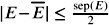 , we conclude E < sep( E ). From the definition of sep( E ), we conclude E = 0.
We have to solve two main problems here. First, we have to find an appropriate separation bound. Second, the evaluation of an approximation E should be as cheap as possible.
The second problem is solved with an iterative approximation process. Rather than computing the approximation within an error bound of ![]() , we increase the precision adaptively until finally the approximation is good enough; see [Burnikel et al. 01]. Let us assume that the separation bound was already computed successfully. The iterative sign test of an expression E with sep( E ) works as follows.
, we increase the precision adaptively until finally the approximation is good enough; see [Burnikel et al. 01]. Let us assume that the separation bound was already computed successfully. The iterative sign test of an expression E with sep( E ) works as follows.
The following is the iterative sign test with separation bound sketch:
-
Initialize by 1;
-
Compute an approximation E of E so that E ˆ E ‰ holds;
-
If E > holds, the sign of E and E coincidence and we are done;
-
Otherwise, from E ‰ we conclude E ‰ 2 . Now we check whether 2 ‰ sep( E ) holds. If this is true, we conclude E = 0 from the definition of the separation bound. Otherwise, we decrease by := /2 and repeat to compute an approximation with respect to .
We adaptively increase the precision. The given iterative test can be implemented in a straightforward manner using an adaptive arithmetic. For example, if we use floating-point arithmetic with arbitrary precision, we will increase the bit length by 1 in every iteration. Obviously, the maximal precision depends on the size of the separation bound and is given by log ( ![]() ) because 2 ‰ sep( E ) is finally fulfilled.
) because 2 ‰ sep( E ) is finally fulfilled.
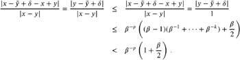
It remains to compute appropriate separation bounds. The computation of a separation bound of an expression E can be represented in an execution table. The execuction table is successively applied to the DAG of the expression and results in a separation bound; see Theorem 9.28. For example, Table 9.3 shows the execution table for a separation bound of algebraic expressions with square roots only; see [Burnikel et al. 00]. Note that many of the standard expressions used in geometric algorithms and presented in Section 9.4.2 do not use arbitrary roots. The presented separation-bound technique is incorporated into data type leda real of the LEDA system; see [Mehlhorn and Nher 00]. For example, if the table is applied to the division-free expression E = ( ![]() ˆ 1)(
ˆ 1)( ![]() + 1) ˆ 1, then we will achieve the bounds u ( E ) = 4 + 2
+ 1) ˆ 1, then we will achieve the bounds u ( E ) = 4 + 2 ![]() and l ( E ) = 1. Applying Theorem 9.28 we can get a separation bound of
and l ( E ) = 1. Applying Theorem 9.28 we can get a separation bound of
for non-zero E . Using precision p = 4, we can conclude that E equals zero.
Theorem 9.28 was proven in [Burnikel et al. 00].
| Expression | u ( E ) | l ( E ) |
|---|---|---|
| Integer n | n | 1 |
| E 1 E 2 | u ( E 1 ) — l ( E 2 ) + u ( E 2 ) — l ( E 1 ) | l ( E 1 ) — l ( E 2 ) |
| E 1 — E 2 | u ( E 1 ) — u ( E 2 ) | l ( E 1 )— l ( E 2 ) |
| E 1 /E 2 | u ( E 1 )— l ( E 2 ) | l ( E 1 )— u ( E 2 ) |
| | | |
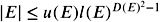
Theorem 9.28. Let E be an algebraic expression with integer input values and operators + , ˆ , /, — , and ![]() . Let k denote the number of
. Let k denote the number of ![]() operations in E and let D ( E ) := 2 k . We can assume that E is represented by a DAG . If we apply the execution table ( Table 9.3 ), we obtain values u ( E ) and l ( E ) such that
operations in E and let D ( E ) := 2 k . We can assume that E is represented by a DAG . If we apply the execution table ( Table 9.3 ), we obtain values u ( E ) and l ( E ) such that
-
 ;
; -
 .
.
If E is division-free then l ( E ) = 1 and D ( E ) 2 can be replaced by D ( E ) .
A comprehensive overview of existing separation bounds, their execution tables, and their analysis can be found in [Li 01]; see also [Burnikel et al. 00, Burnikel et al. 01, Li and Yap 01a].
9.3.4. Exact Geometric Computations (EGC)
EGC combines exact arithmetic or robust adaptive arithmetic with the idea that impreciseness in calculations sometimes can be neglected, whereas the combinatorial structures should always be correct. Thus, it guarantees that all standard geometric algorithms designed for the Real RAM will run as desired; i.e., the flow and the output of the algorithm are correct in a combinatorial sense.
More precisely, in the terminology of EGC intensively considered in [Yap 97a], we differ between constructional steps and combinatorial steps of an algorithm. In the former step, new elements are computed; the latter one causes the algorithm to branch. Different combinatorial steps lead to different computational paths. Each combinatorial step should depend on the evaluation of a geometric predicate. Altogether, to ensure exact combinatorics, it suffices to ensure that all predicates are evaluated exactly. For the numerical part of an algorithm, EGC requires that the result is represented exactly, although it might happen that the exact result can be approximated only within the given arithmetic. For example, we can uniquely represent an intersection of line segments by its endpoints, but the calculation of the coordinates may be erroneous.
Summarizing the EGC approach requires that
-
the algorithm is driven by geometric predicates only,
-
geometric expressions are represented uniquely, and
-
the sign of a geometric predicate is evaluated correctly.
EGC is sort of a paradigm that can be fulfilled by many approaches. We have to ensure that the underlying arithmetic produces correct results for the sign of predicates. Therefore, exact integer, rational, or algebraic arithmetic is suitable. But also the adaptive approaches of lazy evaluation, separation bounds, floating-point filters, and adaptive floating-point expansions presented in the previous sections may lead to EGC, provided that the precision can be adapted adequately.
The idea of EGC is well supported by the CGAL library; see [Overmars 96], which is a C++ library of geometric algorithms and data structures. The corresponding algorithms are designed under the Real RAM model, and the flow of the algorithms are driven by geometric predicates. Therefore, we can combine CGAL with an arbitrary number package that fulfills the ECG paradigm. For example, we can make use of exact multi-precision rationals or floats of the C++ package GMP, or we can use adaptive arithmetic realized in the C++ library LEDA; see [Mehlhorn and Nher 00], which is based on floating-point filters, separation bounds, and algebraic numbers; see also [Burnikel et al. 95], [Karamcheti et al. 99a], [Li and Yap 01b], and [Li 01].
EAN: N/A
Pages: 69
- Chapter I e-Search: A Conceptual Framework of Online Consumer Behavior
- Chapter III Two Models of Online Patronage: Why Do Consumers Shop on the Internet?
- Chapter VIII Personalization Systems and Their Deployment as Web Site Interface Design Decisions
- Chapter XII Web Design and E-Commerce
- Chapter XIV Product Catalog and Shopping Cart Effective Design